|
|
|
|
|

1. Abstract
OPAL is a parallel open source tool for charged-particle optics in linear accelerators and rings, including 3D space charge. Using the MAD language with extensions, OPAL can run on a laptop as well as on the largest high performance computing systems. OPAL is built from the ground up as a parallel application exemplifying the fact that high performance computing is the third leg of science, complementing theory and experiment.
The OPAL framework makes it easy to add new features in the form of new C++ classes. OPAL comes in the following flavours:
- OPAL-cycl
-
tracks particles with 3D space charge including neighbouring turns in cyclotrons and FFAs with time as the independent variable.
- OPAL-t
-
models beam lines, linacs, rf-photo injectors and complete XFELs.
- OPAL-map
-
map tracking (experimental, no space charge yet)
It should be noted that not all features of OPAL are available in all flavours.
2. Introduction
2.1. History
Using the MAD language with extensions, OPAL is derived from MAD9P and is based on the CLASSIC [1] class library, which was started in 1995 by an international collaboration. IPPL (Independent Parallel Particle Layer) is the framework which provides parallel particles and fields using data parallel approach. IPPL was inspired by the POOMA [6].
OPAL-t can be used to model guns, injectors, ERLs and complete XFELs.
2.2. Parallel Processing Capabilities
OPAL is built to harness the power of parallel processing for an improved quantitative understanding of particle accelerators. This goal can only be achieved with detailed 3D modelling capabilities and a sufficient number of simulation particles to obtain meaningful statistics on various quantities of the particle ensemble such as emittance, slice emittance, halo extension etc.
The following example is exemplifying this fact:
| Distribution | Particles | Mesh | Greens Function | Time steps |
|---|---|---|---|---|
Gauss 3D |
\(10^8\) |
\(1024^3\) |
Integrated |
10 |
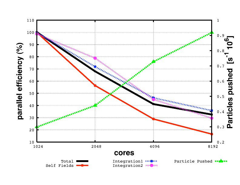
Figure 1 shows the parallel efficiency time as a function of used cores for a test example with parameters given in Table 1. The data were obtained on a Cray XT5 at the Swiss Center for Scientific Computing.
2.3. Quality Management
Documentation and quality assurance are given our highest attention since we are convinced that adequate documentation is a key factor in the usefulness of a code like OPAL to study present and future particle accelerators. Using tools such as a source code version control system (git), source code documentation using Doxygen (found here) and the extensive user manual you are now enjoying, we are committed to providing users as well as co-developers with state-of-the-art documentation to OPAL.
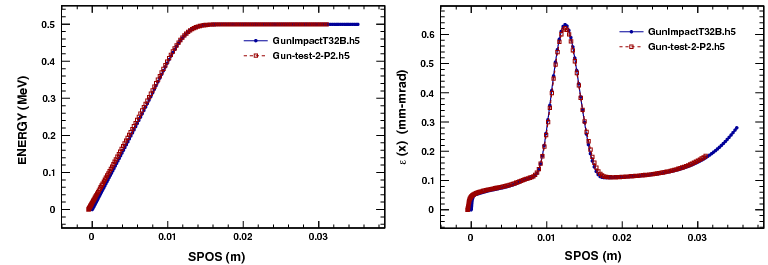
One example of an non trivial test-example is the PSI DC GUN. In Figure 2 the comparison between Impact-t and OPAL-t is shown. This example is part of the regression test suite that is run every night. The input file is found in Examples of Particle Accelerators and Beamlines.
Misprints and obscurity are almost inevitable in a document of this size. Comments and active contributions from readers are therefore most welcome. They may be sent to Andreas Adelmann.
2.4. Output
The phase space is stored in the H5hut file-format [3]
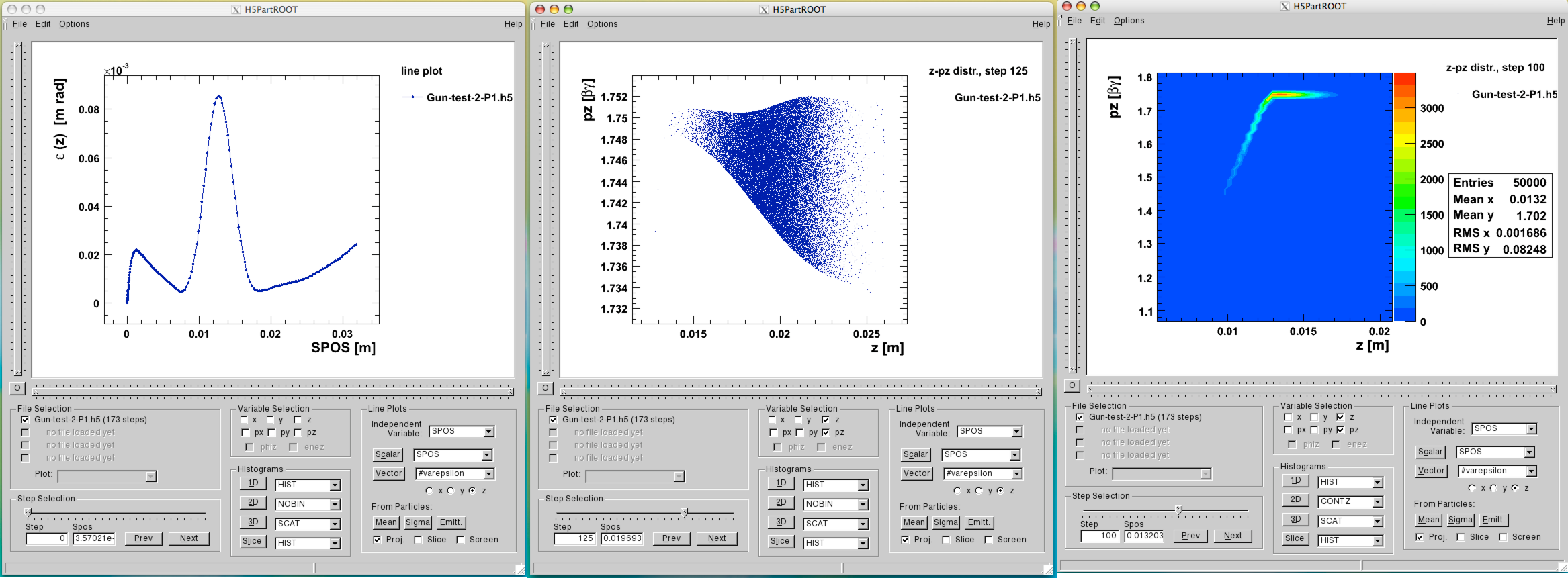
and can be analyzed using e.g. H5root [4], [5].
The frequency of the data output (phase space and some statistical quantities)
can be controlled using the (see Option Statement),
with the flag PSDUMPFREQ. The file is named like in input file but with the extension .h5.
A SDDS compatible ASCII file with statistical beam parameters is written
to a file with extension .stat. The frequency with which this data is
written can be controlled with the OPTION statement
with the flag STATDUMPFREQ.
For postprocessing we recommend to use the pyOPALTools Python package which contains many tools for pre- and postprocessing, and analysing and plotting output data.
In addition to the output files, note that important information is displayed on the stdout i.e. the terminal. The user is advised to consult the stdout frequently.
2.5. Change History
See Release Notes for a detailed list of changes in OPAL.
2.6. Known Issues and Limitations
See the issue list in the repository.
See also pitfalls and limitations.
2.7. Acknowledgments
The contributions of various individuals and groups are acknowledged in the relevant chapters, however a few individuals have or had considerable influence on the development of OPAL, namely Chris Iselin, John Jowett, Julian Cummings, Ji Qiang, Robert Ryne and Stefan Adam. For the H5root visualization tool credits go to Thomas Schietinger.
The following individuals are acknowledged for past contributions: Christian Baumgarten, J. Scott Berg, Yuanjie Bi, David Bruhwiler, Chris Cortes, Martin Duy Tat, Philippe Ganz, Colwyn Gulliford, Yves Ineichen, Tulin Kaman, Christopher Mayes, Xiaoying Pang, Valeria Rizzoglio, Chuan Wang, Jianjun Yang, Hao Zha.
2.8. Citation
Please cite OPAL in the following way:
@ARTICLE{2019arXiv190506654A,
       author = {{Adelmann}, Andreas and {Calvo}, Pedro and {Frey}, Matthias and
         {Gsell}, Achim and {Locans}, Uldis and {Metzger-Kraus}, Christof and
         {Neveu}, Nicole and {Rogers}, Chris and {Russell}, Steve and
         {Sheehy}, Suzanne and {Snuverink}, Jochem and {Winklehner}, Daniel},
        title = "{OPAL a Versatile Tool for Charged Particle Accelerator Simulations}",
      journal = {arXiv e-prints},
     keywords = {Physics - Accelerator Physics},
         year = "2019",
        month = "May",
          eid = {arXiv:1905.06654},
        pages = {arXiv:1905.06654},
archivePrefix = {arXiv},
       eprint = {1905.06654},
 primaryClass = {physics.acc-ph},
       adsurl = {https://ui.adsabs.harvard.edu/abs/2019arXiv190506654A},
      adsnote = {Provided by the SAO/NASA Astrophysics Data System}
}
2.9. References
[1] F. C. Iselin, The classic project, Tech. Rep. CERN/SL/96-061, European Organization for Nuclear Research (1996).
[2] J. Qiang et al., A three-dimensional quasi-static model for high brightness beam dynamics simulation, Tech. Rep. LBNL-59098, Lawrence Berkeley National Laboratory (2005).
[3] M. Howison et al., H5hut: A High-Performance I/O Library for Particle-based Simulations, in 2010 IEEE International Conference on Cluster Computing Workshops and Posters, vol. 1, pp. 1–8 (Heraklion, Crete, 2010).
[5] T. Schietinger, H5PartROOT - A visualization and post-processing tool for accelerator simulations, in Proceedings of the 10th International Computational Accelerator Physics conference (ICAP09), pp. 343-346 (San Francisco, CA, USA, 2009).
[6] R. Günther, Parallel Object-Oriented Methods and Applications (2005).
3. Conventions
3.1. Physical Units
Throughout the computations OPAL uses international units, as defined by SI (Système International).
| Quantity | Dimension |
|---|---|
Length |
\(\mathrm{m}\) (meters) |
Angle |
\(\mathrm{rad}\) (radians) |
Quadrupole coefficient |
\(\mathrm{Tm^{-1}}\) |
Multipole coefficient, 2n poles |
\(\mathrm{Tm^{-n + 1}}\) |
Electric voltage |
\(\mathrm{MV}\) (Megavolts) |
Electric field strength |
\(\mathrm{MV m^{-1}}\) |
Frequency |
\(\mathrm{MHz}\) (Megahertz) |
Particle energy |
\(\mathrm{MeV}\) or \(\mathrm{eV}\) |
Particle mass |
\(\mathrm{MeV c^{-2}}\) |
Particle momentum |
\(\mathrm{\beta\gamma}\) or \(\mathrm{eV}\) |
Beam current |
\(\mathrm{A}\) (Amperes) |
Particle charge |
\(\mathrm{e}\) (elementary charges) |
Impedances |
\(\mathrm{M \Omega}\) (Megaohms) |
Emittances (normalized and geometric |
\(\mathrm{mrad}\) |
RF power |
\(\mathrm{MW}\) (Megawatts) |
3.2. OPAL-cycl
The OPAL-cycl flavor see Cyclotron is using the so called
Cyclotron units. Lengths are defined in (mm), frequencies in (MHz), momenta
in (\(\beta\gamma\)) and angles in (deg), except RFPHI which
is in (rad).
3.3. Symbols used
| Symbol | Definition |
|---|---|
\(X\) |
Ellipse axis along the \(x\) dimension [m]. \(X=R\) for circular beams. |
\(Y\) |
Ellipse axis along the \(y\) dimension [m]. \(Y=R\) for circular beams. |
\(R\) |
Beam radius for circular beam [m]. |
\(R^*\) |
Effective beam radius for elliptical beam: \(R^* = (X+Y)/2\) [m]. |
\(\sigma_x\) |
Rms beam size in \(x\): \(\sigma_x = \langle x^2\rangle^{1/2}\) [m]. \(\sigma_x = X/2\) for elliptical or circular beams (X=Y=R). |
\(\sigma_y\) |
Rms beam size in \(y\): \(\sigma_y = \langle y^2\rangle^{1/2}\) [m]. \(\sigma_y = Y/2\) for elliptical or circular beams (X=Y=R). |
\(\sigma_i\) |
Rms beam size in \(x\) (i=1) or \(y\) (i=2): \(\sigma=\langle x^2\rangle^{1/2}\) or \(\langle y^2\rangle^{1/2}\) [m]. |
\(\sigma_L\) |
Rms beam size in the Larmor frame for cylindrical symmetric beam and external fields [m]: \(\sigma_L = \sigma_x = \sigma_y\). |
\(\sigma_r\) |
Rms beam size in \(r\) for a circular beam: \(\sigma_r =\langle r^2\rangle^{1/2} = R/\sqrt{2}\) [m]. |
\(\sigma^*\) |
Average rms size for elliptical beam: \(\sigma^* = (\sigma_x+\sigma_y)/2\) [m]. |
\(\theta_r\) |
Larmor angle [rad] |
\(\dot\theta_r\) |
Time derivative of Larmor angle: \(\dot\theta_r = -eB_z/2m\gamma\) [rad/sec]. |
\(z_s\) |
Longitudinal position of a particular beam slice [m]. |
\(z_h,z_t\) |
Position of the head & tail of a beam bunch [m]. |
\(\zeta\) |
Used to label the position of a beam slice in the beam [m]. For bunched beams: \(\zeta = z_s-z_t\). |
\(\xi\) |
Used to label the position of a slice image charge [m]. For bunched beams: \(\xi = z_h + z_t\). |
\(K\) |
Focusing function of cylindrical symmetric external fields: \(K = -\frac{\partial F_r}{\partial r}\) [N/m]. |
\(K_i\) |
Focusing function in \(x_i\) direction: \(K_i = -\frac{\partial F_{x_i}}{\partial x_i}\) [N/m]. |
\(I_0\) |
Alfven current: \(I_0= e/4\pi\epsilon_0mc^3\) [A]. |
\(I\) |
Beam current [A]. |
\(I(\zeta)\) |
Slice beam current [A]. |
\(k_p\) |
Beam perveance: \(k_p = I(\zeta)/2I_0\) |
\(g(\zeta)\) |
Form factor used in slice analysis of bunched beams. |
4. Pitfalls and Limitations
A loose collection of pitfalls that may be difficult to avoid in particular for new users but also experienced user might profit from this list.
4.1. Hard Edge Fields
Fields that feature steps like hard edge fringe fields are strongly advised not to be used. In sector magnets where particles have different path lengths inside the magnet they are kicked 1, 2 or even more steps more (or less) depending on position and momentum. Combine it with big time steps and you’ll observe strange effects like splitting beams.
4.2. Very Short Active Elements / Big Time Steps
This is similar to the problem with hard edge fields. This concerns elements that model electromagnetic devices whose lengths are very short and comparable to the time step. In this case a split of the bunch can be observed which is caused by the fact that some particles are kicked more often than others. The length of the time step should then be decreased to reduce this effect.
5. Tutorial
This chapter will provide a jump start describing some of the most common used features of OPAL. The complete set of examples can be found and downloaded at https://gitlab.psi.ch/OPAL/src/wikis/home. All examples are requiring a small amount of computing resources and run on a single core, but can be used efficiently on up to 8 cores. OPAL scales in the weak sense, hence for a higher concurrency one has to increase the problem size i.e. number of macro particles and the grid size, which is beyond this tutorial.
5.1. The Simulation Cycle
5.2. Starting OPAL
The name of the application is opal. When called without any argument
an interactive session is started.
\$ opal
Ippl> CommMPI: Parent process waiting for children ...
Ippl> CommMPI: Initialization complete.
>                ____  _____       ___
>               / __ \|  __ \ /\   | |
>              | |  | | |__) /  \  | |
>              | |  | |  ___/ /\ \ | |
>              | |__| | |  / ____ \| |____
>               \____/|_| /_/    \_\______|
OPAL >
OPAL > This is OPAL (Object Oriented Parallel Accelerator Library) Version 2.0.0 ...
OPAL >
OPAL > Please send cookies, goodies or other motivations (wine and beer ... )
OPAL > to the OPAL developers opal@lists.psi.ch
OPAL >
OPAL > Time: 16.43.23 date: 30/05/2017
OPAL > Reading startup file "/Users/adelmann/init.opal".
OPAL > Finished reading startup file.
==>
One can exit from this session with the command QUIT; (including the
semicolon).
For batch runs OPAL accepts the following command line arguments:
| Argument | Values | Function |
|---|---|---|
--input |
<file > |
the input file. Using "--input" is optional. Instead the input file can be provided either as first or as last argument. |
--info |
0 – 5 |
controls the amount of output to the command line. 0
means no or scarce output, 5 means a lot of output. Default: 1. |
--restart |
-1 – <Integer> |
restarts from given step in file with saved phase space. Per default OPAL tries to restart from a file <file>.h5 where <file>is the input file without extension. -1 stands for the last step in the file. If no other file is specified to restart from and if the last step of the file is chosen, then the new data is appended to the file. Otherwise the data from this particular step is copied to a new file and all new data appended to the new file. |
--restartfn |
<file> |
a file in H5hut format from which OPAL should restart. |
--help |
Displays a summary of all command-line arguments and then quits. |
|
--version |
Prints the version and then quits. |
Example:
opal input.in --restartfn input.h5 --restart -1 --info 3
5.3. Auto-phase Example
This is a partially complete example. First we have to set OPAL in
AUTOPHASE mode, as described in Option Statement and for example set
the nominal phase to \(-3.5^{\circ}\)). The way how OPAL is
computing the phases is explained in Appendix Auto-phasing Algorithm.
Option, AUTOPHASE=4;

REAL FINSS_RGUN_phi= (-3.5/180*Pi);
The cavity would be defined like
FINSS_RGUN: RFCavity, L = 0.17493, VOLT = 100.0,
    FMAPFN = "FINSS-RGUN.dat",
    ELEMEDGE =0.0, TYPE = "STANDING", FREQ = 2998.0,
    LAG = FINSS_RGUN_phi;
with FINSS_RGUN_phi defining the off crest phase. Now a normal TRACK
command can be executed. A file containing the values of maximum phases
is created, and has the format like:
1
FINSS_RGUN
2.22793
with the first entry defining the number of cavities in the simulation.
5.4. Examples of Particle Accelerators and Beamlines
5.4.1. Laser emission, OBLA (SwissFEL test facility) 4 MeV Gun and Beamline
All supplementary files can be found in the laser emission regression test.
5.4.2. PSI Injector II Cyclotron
Injector II is a separated sector cyclotron specially designed for pre-acceleration (inject: 870 keV, extract: 72 MeV) of high intensity proton beam for Ring cyclotron. It has 4 sector magnets, two double-gap acceleration cavities (represented by 2 single-gap cavities here) and two single-gap flat-top cavities.
Following is an input file of Single Particle Tracking mode for PSI Injector II cyclotron.
The supplementary files should be placed in the same directory.
To run opal on a single node, just use this command:
opal Injector2.in
Here shows some pictures using the resulting data from single particle tracking using OPAL-cycl.
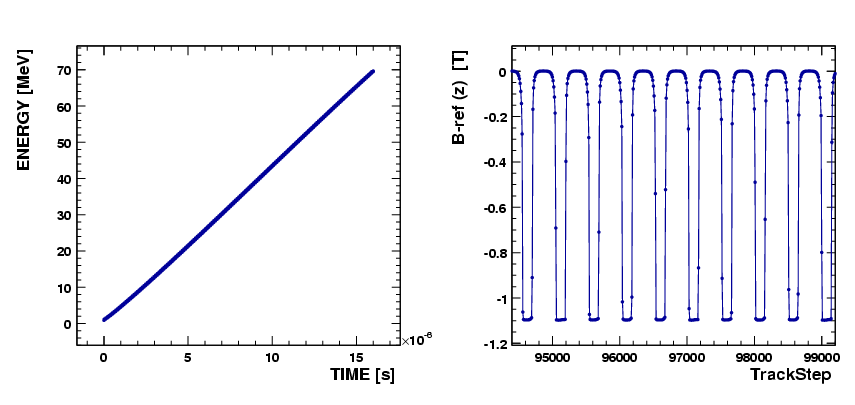
Left plot of Figure 5 shows the accelerating orbit of reference particle. After 106 turns, the energy increases from 870 keV at the injection point to 72.16 MeV at the deflection point.
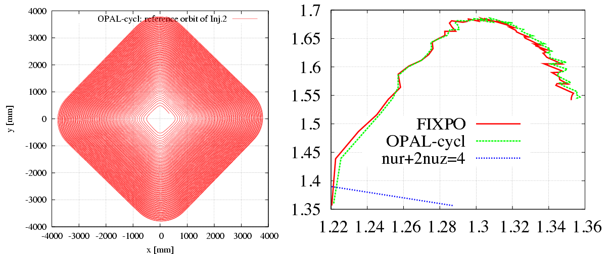
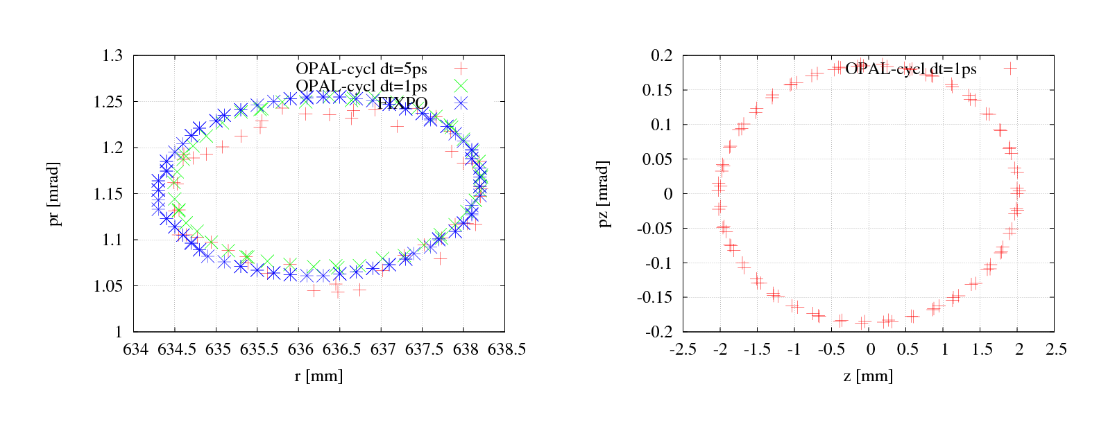
From theoretic view, there should be an eigen ellipse for any given energy in stable area of a fixed accelerator structure. Only when the initial phase space shape matches its eigen ellipse, the oscillation of beam envelop amplitude will get minimal and the transmission efficiency get maximal. We can calculate the eigen ellipse by single particle tracking using betatron oscillation property of off-centered particle as following: track an off-centered particle and record its coordinates and momenta at the same azimuthal position for each revolution. Figure 6 shows the eigen ellipse at symmetric line of sector magnet for energy of 2 MeV in Injector II.
Right plot of Figure 5 shows very good agreement of the tune diagram by OPAL-cycl and FIXPO. The trivial discrepancy should come from the methods they used. In FIXPO, the tune values are obtained according to the crossing points of the initially displaced particle. Meanwhile, in OPAL-cycl, the Fourier analysis method is used to manipulate orbit difference between the reference particle and an initially displaced particle. The frequency point with the biggest amplitude is the betatron tune value at the given energy.
Following is the input file for single bunch tracking with space charge effects in Injector II.
For the supplementary files see above, PSI Injector II Cyclotron
To run opal on single node, just use this command:
opal Injector2-sc.in
To run opal on N nodes in parallel environment interactively, use this command instead:
mpirun -np N opal Injector2-sc.in
If restart a job from the last step of an existing .h5 file, add a new argument like this:
mpirun -np N opal Injector2-sc.in --restart -1
5.4.3. PSI Ring Cyclotron
From the view of numerical simulation, the difference between Injector II and Ring cyclotron comes from two aspects:
- B Field
-
The structure of Ring is totally symmetric, the field on median plain is periodic along azimuthal direction, OPAL-cycl take this advantage to only store field data to save memory.
- RF Cavity
-
In the Ring, all the cavities are typically single gap with some parallel displacement from its radial position.OPAL-cycl have an argument
PDISto manipulate this issue.
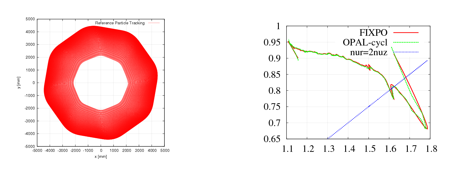
Figure 9 shows a single particle tracking result and tune calculation result in the PSI Ring cyclotron. Limited by size of the user guide, we don’t plan to show too much details as in Injector II.
5.5. Translate Old to New Distribution Commands
As of OPAL 1.2, the distribution command see Chapter Distribution was changed significantly. Many of the changes were internal to the code, allowing us to more easily add new distribution command options. However, other changes were made to make creating a distribution easier, clearer and so that the command attributes were more consistent across distribution types. Therefore, we encourage our users to refer to when creating any new input files, or if they wish to update existing input files.
With the new distribution command, we did attempt as much as possible to make it backward compatible so that existing OPAL input files would still work the same as before, or with small modifications. In this section of the manual, we will give several examples of distribution commands that will still work as before, even though they have antiquated command attributes. We will also provide examples of commonly used distribution commands that need small modifications to work as they did before.
An important point to note is that it is very likely you will see small changes in your simulation even when the new distribution command is nominally generating particles in exactly the same way. This is because random number generators and their seeds will likely not be the same as before. These changes are only due to OPAL using a different sequence of numbers to create your distribution, and not because of errors in the calculation. (Or at least we hope not.)
5.5.1. GUNGAUSSFLATTOPTH and ASTRAFLATTOPTH Distribution Types
The GUNGAUSSFLATTOPTH and
ASTRAFLATTOPTH
distribution types are two
common types previously implemented to simulate electron beams emitted
from photocathodes in an electron photoinjector. These are no longer
explicitly supported and are instead now defined as specialized
sub-types of the distribution type FLATTOP. That is, the emitted
distributions represented by GUNGAUSSFLATTOPTH and ASTRAFLATTOPTH
can now be easily reproduced by using the FLATTOP distribution type
and we would encourage use of the new command structure.
Having said this, however, old input files that use the
GUNGAUSSFLATTOPTH and ASTRAFLATTOPTH distribution types will still
work as before, with the following exception. Previously, OPAL had a
Boolean OPTION command FINEEMISSION (default value was TRUE). This
OPTION is no longer supported. Instead you will need to set the
distribution attribute Table 20 to a
value that is 10 \(\times\) the value of the distribution
attribute Table 18 in order for your
simulation to behave the same as before.
5.5.2. FROMFILE, GAUSS and BINOMIAL Distribution Types
5.5.3. Change in Momentum Units
Input momentum can be given without units i.e. as \(\beta\gamma\), or in eV/c. Up until OPAL 2.2 eV was used instead of eV/c, but this was changed since eV is a unit of energy rather than momentum. To adapt old files with momentum in eV, such that they can work for the newer OPAL versions, the following formula can be used:
and you will need to set the distribution attribute
INPUTMOUNITS to:
INPUTMOUNITS = EVOVERC
6. OPAL-t
6.1. Introduction
OPAL-t is a fully three-dimensional program to track in time, relativistic particles taking into account space charge forces, self-consistently in the electrostatic approximation, and short-range longitudinal and transverse wake fields. OPAL-t is one of the few codes that is implemented using a parallel programming paradigm from the ground up. This makes OPAL-t indispensable for high statistics simulations of various kinds of existing and new accelerators. It has a comprehensive set of beamline elements, and furthermore allows arbitrary overlap of their fields, which gives OPAL-t a capability to model both the standing wave structure and traveling wave structure. Beside IMPACT-T it is the only code making use of space charge solvers based on an integrated Green [7], [8], [9] function to efficiently and accurately treat beams with large aspect ratio, and a shifted Green function to efficiently treat image charge effects of a cathode [10], [7], [8],[9]. For simulations of particles sources i.e. electron guns OPAL-t uses the technique of energy binning in the electrostatic space charge calculation to model beams with large energy spread. In the very near future a parallel Multigrid solver taking into account the exact geometry will be implemented.
6.2. Variables in OPAL-t
OPAL-t uses the following canonical variables to describe the motion of particles. The physical units are listed in square brackets.
- X
-
Horizontal position \(x\) of a particle relative to the axis of the element [m].
- PX
-
\(\beta_x\gamma\) Horizontal canonical momentum [Units].
- Y
-
Vertical position \(y\) of a particle relative to the axis of the element [m].
- PY
-
\(\beta_y\gamma\) Vertical canonical momentum [Units].
- Z
-
Longitudinal position \(z\) of a particle in floor co-ordinates [m].
- PZ
-
\(\beta_z\gamma\) Longitudinal canonical momentum [Units].
The independent variable is t [s].
6.3. Integration of the Equation of Motion
OPAL-t integrates the relativistic Lorentz equation
where \(\gamma\) is the relativistic factor, \(q\) is the charge, and \(m\) is the rest mass of the particle. \(\mathbf{E}\) and \(\mathbf{B}\) are abbreviations for the electric field \(\mathbf{E}(\mathbf{x},t)\) and magnetic field \(\mathbf{B}(\mathbf{x},t)\). To update the positions and momenta OPAL-t uses the Boris-Buneman algorithm [11].
6.4. Positioning of Elements
Since OPAL version 2.0 of OPAL elements can be placed in space using
3D coordinates X, Y, Z, THETA, PHI and PSI, see
Common Attributes for all Elements.
The old notation using ELEMEDGE is still
supported. OPAL-t then computes the position in 3D using ELEMDGE,
ANGLE and DESIGNENERGY. It assumes that the trajectory consists of
straight lines and segments of circles. Fringe fields are ignored. For
cases where these simplifications aren’t justifiable the user should use
3D positioning. For a simple switchover OPAL writes a file _3D.opal
where all elements are placed in 3D.
Beamlines containing guns should be supplemented with the element
SOURCE. This allows OPAL to distinguish the cases and adjust the
initial energy of the reference particle.
Prior to OPAL version 2.0 elements needed only a defined length. The transverse extent was not defined for elements except when combined with 2D or 3D field maps. An aperture had to be designed to give elements a limited extent in transverse direction since elements now can be placed freely in three-dimensional space. See Common Attributes for all Elements for how to define an aperture.
6.5. Coordinate Systems
The motion of a charged particle in an accelerator can be described by relativistic Hamilton mechanics. A particular motion is that of the reference particle, having the central energy and traveling on the so-called reference trajectory. Motion of a particle close to this fictitious reference particle can be described by linearized equations for the displacement of the particle under study, relative to the reference particle. In OPAL-t, the time \(t\) is used as independent variable instead of the path length \(s\). The relation between them can be expressed as
6.5.1. Global Cartesian Coordinate System
We define the global cartesian coordinate system, also known as floor coordinate system with \(K\), a point in this coordinate system is denoted by \((X, Y, Z) \in K\). In Figure 10 of the accelerator is uniquely defined by the sequence of physical elements in \(K\). The beam elements are numbered \(e_0, \ldots , e_i, \ldots e_n\).
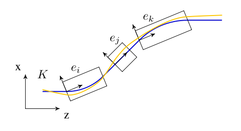
6.5.2. Local Cartesian Coordinate System
A local coordinate system \(K'_i\) is attached to each element \(e_i\). This is simply a frame in which \((0,0,0)\) is at the entrance of each element. For an illustration see Figure 10. The local reference system \((x, y, z) \in K'_n\) may thus be referred to a global Cartesian coordinate system \((X, Y, Z) \in K\).
The local coordinates \((x_i, y_i, z_i)\) at element \(e_i\) with respect to the global coordinates \((X, Y, Z)\) are defined by three displacements \((X_i, Y_i, Z_i)\) and three angles \((\Theta_i, \Phi_i, \Psi_i)\).
\(\Psi\) is the roll angle about the global \(Z\)-axis. \(\Phi\) is the yaw angle about the global \(Y\)-axis. Lastly, \(\Theta\) is the pitch angle about the global \(X\)-axis. All three angles form right-handed screws with their corresponding axes. The angles (\(\Theta,\Phi,\Psi\)) are the Tait-Bryan angles [12].
The displacement is described by a vector \(\mathbf{v}\) and the orientation by a unitary matrix \(\mathcal{W}\). The column vectors of \(\mathcal{W}\) are unit vectors spanning the local coordinate axes in the order \((x, y, z)\). \(\mathbf{v}\) and \(\mathcal{W}\) have the values:
where
We take the vector \(\mathbf{r}_i\) to be the displacement and the matrix \(\mathcal{S}_i\) to be the rotation of the local reference system at the exit of the element \(i\) with respect to the entrance of that element.
Denoting with \(i\) a beam line element, one can compute \(\mathbf{v}_i\) and \(\mathcal{W}_i\) by the recurrence relations
where
\(\mathbf{v}_0\) corresponds to the origin of the LINE and
\(\mathcal{W}_0\) to its orientation. In OPAL-t they can be
defined using either X, Y, Z, THETA, PHI and PSI or ORIGIN
and ORIENTATION, see Simple Beam Lines.
6.5.3. Space Charge Coordinate System
In order to calculate space charge in the electrostatic approximation, we introduce a co-moving coordinate system \(K_{\text{sc}}\), in which the origin coincides with the mean position of the particles and the mean momentum is parallel to the z-axis.
6.5.4. Curvilinear Coordinate System
In order to compute statistics of the particle ensemble, \(K_s\) is introduced. The accompanying tripod (Dreibein) of the reference orbit spans a local curvilinear right handed system \((x,y,s)\). The local \(s\)-axis is the tangent to the reference orbit. The two other axes are perpendicular to the reference orbit and are labelled \(x\) (in the bend plane) and \(y\) (perpendicular to the bend plane).
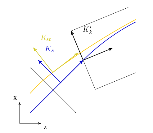
Both coordinate systems are described in Figure 11.
6.5.5. Design or Reference Orbit
The reference orbit consists of a series of straight sections and circular arcs and is computed by the Orbit Threader i.e. deduced from the element placement in the floor coordinate system.
6.5.6. Compatibility Mode
To facilitate the change for users we will provide a compatibility mode.
The idea is that the user does not have to change the input file.
Instead OPAL-t will compute the positions of the elements. For this it
uses the bend angle and chord length of the dipoles and the position of
the elements along the trajectory. The user can choose whether effects
due to fringe fields are considered when computing the path length of
dipoles or not. The option to toggle OPAL-t’s behavior is called
IDEALIZED. OPAL-t assumes per default that provided ELEMEDGE for
elements downstream of a dipole are computed without any effects due to
fringe fields.
Elements that overlap with the fields of a dipole have to be handled separately by the user to position them in 3D.
We split the positioning of the elements into two steps. In a first step we compute the positions of the dipoles. Here we assume that their fields don’t overlap. In a second step we can then compute the positions and orientations of all other elements.
The accuracy of this method is good for all elements except for those that overlap with the field of a dipole.
6.5.7. Orbit Threader and Autophasing
The OrbitThreader integrates a design particle through the lattice and
setups up a multi map structure (IndexMap). Furthermore when the
reference particle hits an rf-structure for the first time then it
auto-phases the rf-structure, see Appendix Auto-phasing Algorithm. The multi map
structure speeds up the search for elements that influence the particles
at a given position in 3D space by minimizing the looping over elements
when integrating an ensemble of particles. For each time step,
IndexMap returns a set of elements
\(\mathcal{S}_{\text{e}} \subset {e_0 \ldots e_n}\) in case of
the example given in Figure 10. An implicit drift is modelled as an
empty set \(\emptyset\).
6.6. Flow Diagram of OPAL-t
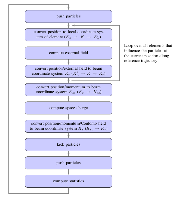
A regular time step in OPAL-t is sketched in Figure 12. In order to compute the coordinate system transformation from the reference coordinate system \(K_s\) to the local coordinate systems \(K'_n\) we join the transformation from floor coordinate system \(K\) to \(K'_n\) to the transformation from \(K_s\) to \(K\). All computations of rotations which are involved in the computation of coordinate system transformations are performed using quaternions. The resulting quaternions are then converted to the appropriate matrix representation before applying the rotation operation onto the particle positions and momenta.
As can be seen from Figure 12 the integration of the trajectories of the particles are integrated and the computation of the statistics of the six-dimensional phase space are performed in the reference coordinate system.
6.7. Output
In addition to the progress report that OPAL-t writes to the standard output (stdout) it also writes different files for various purposes.
6.7.1. <input_file_name >.stat
This file is used to log the statistical properties of the bunch in the
ASCII variant of the SDDS format [13]. It can be viewed
with the SDDS Tools [14] or GNUPLOT. The frequency with
which the statistics are computed and written to file can be controlled
With the option STATDUMPFREQ. The information that is stored are found
in the following table.
| Column Nr. | Name | Units | Meaning |
|---|---|---|---|
1 |
t |
ns |
Time |
2 |
s |
m |
Path length |
3 |
numParticles |
1 |
Number of macro particles |
4 |
charge |
C |
Bunch charge |
5 |
energy |
MeV |
Mean bunch energy |
6 |
rms_x |
m |
RMS beamsize in x |
7 |
rms_y |
m |
RMS beamsize in y |
8 |
rms_s |
m |
RMS beamsize in s |
9 |
rms_px |
1 |
RMS beamsize normalised momentum in x |
10 |
rms_py |
1 |
RMS beamsize normalised momentum in y |
11 |
rms_ps |
1 |
RMS beamsize normalised momentum in s |
12 |
emit_x |
mrad |
Normalized emittance in x |
13 |
emit_y |
mrad |
Normalized emittance in y |
14 |
emit_s |
mrad |
Normalized emittance in s |
15 |
mean_x |
m |
X-component of mean position relative to reference particle |
16 |
mean_y |
m |
Y-component of mean position relative to reference particle |
17 |
mean_s |
m |
S-component of mean position relative to reference particle |
18 |
ref_x |
m |
X-component of reference particle in floor coordinate system |
19 |
ref_y |
m |
Y-component of reference particle in floor coordinate system |
20 |
ref_z |
m |
Z-component of reference particle in floor coordinate system |
21 |
ref_px |
1 |
X-component of normalized momentum of reference particle in floor coordinate system |
22 |
ref_py |
1 |
Y-component of normalized momentum of reference particle in floor coordinate system |
23 |
ref_pz |
1 |
Z-component of normalized momentum of reference particle in floor coordinate system |
24 |
max_x |
m |
Max beamsize in x-direction |
25 |
max_y |
m |
Max beamsize in y-direction |
26 |
max_s |
m |
Max beamsize in s-direction |
27 |
xpx |
1 |
Correlation between x-components of positions and momenta |
28 |
ypy |
1 |
Correlation between y-components of positions and momenta |
29 |
zpz |
1 |
Correlation between s-components of positions and momenta |
30 |
Dx |
m |
Dispersion in x-direction |
31 |
DDx |
1 |
Derivative of dispersion in x-direction |
32 |
Dy |
m |
Dispersion in y-direction |
33 |
DDy |
1 |
Derivative of dispersion in y-direction |
34 |
Bx_ref |
T |
X-component of magnetic field at reference particle |
35 |
By_ref |
T |
Y-component of magnetic field at reference particle |
36 |
Bz_ref |
T |
Z-component of magnetic field at reference particle |
37 |
Ex_ref |
MVm^-1 |
X-component of electric field at reference particle |
38 |
Ey_ref |
MVm^-1 |
Y-component of electric field at reference particle |
39 |
Ez_ref |
MVm^-1 |
Z-component of electric field at reference particle |
40 |
dE |
MeV |
Energy spread of the bunch |
41 |
dt |
ns |
Size of time step |
42 |
partsOutside |
1 |
Number of particles outside
\(n \times gma\) of beam, where \(n\) is controlled
with |
43 |
R0_x |
m |
X-component of position of particle with ID 0 (only when run serial) |
44 |
R0_y |
m |
Y-component of position of particle with ID 0 (only when run serial) |
45 |
R0_s |
m |
S-component of position of particle with ID 0 (only when run serial) |
46 |
P0_x |
m |
X-component of momentum of particle with ID 0 (only when run serial) |
47 |
P0_y |
m |
Y-component of momentum of particle with ID 0 (only when run serial) |
48 |
P0_s |
m |
S-component of momentum of particle with ID 0 (only when run serial) |
6.7.2. data/<input_file_name >_Monitors.stat
OPAL-t computes the statistics of the bunch for every MONITOR that
it passes. The information that is written can be found in the following
table.
| Column Nr. | Name | Units | Meaning |
|---|---|---|---|
1 |
name |
a string |
Name of the monitor |
2 |
s |
m |
Position of the monitor in path length |
3 |
t |
ns |
Time at which the reference particle pass |
4 |
numParticles |
1 |
Number of macro particles |
5 |
rms_x |
m |
Standard deviation of the x-component of the particles positions |
6 |
rms_y |
m |
Standard deviation of the y-component of the particles positions |
7 |
rms_s |
m |
Standard deviation of the s-component of the particles
positions (only nonvanishing when type of |
8 |
rms_t |
ns |
Standard deviation of the passage time of the particles
(zero if type is of |
9 |
rms_px |
1 |
Standard deviation of the x-component of the particles momenta |
10 |
rms_py |
1 |
Standard deviation of the y-component of the particles momenta |
11 |
rms_ps |
1 |
Standard deviation of the s-component of the particles momenta |
12 |
emit_x |
mrad |
X-component of the normalized emittance |
13 |
emit_y |
mrad |
Y-component of the normalized emittance |
14 |
emit_s |
mrad |
S-component of the normalized emittance |
15 |
mean_x |
m |
X-component of mean position relative to reference particle |
16 |
mean_y |
m |
Y-component of mean position relative to reference particle |
17 |
mean_s |
m |
S-component of mean position relative to reference particle |
18 |
mean_t |
ns |
Mean time at which the particles pass |
19 |
ref_x |
m |
X-component of reference particle in floor coordinate system |
20 |
ref_y |
m |
Y-component of reference particle in floor coordinate system |
21 |
ref_z |
m |
Z-component of reference particle in floor coordinate system |
22 |
ref_px |
1 |
X-component of normalized momentum of reference particle in floor coordinate system |
23 |
ref_py |
1 |
Y-component of normalized momentum of reference particle in floor coordinate system |
24 |
ref_pz |
1 |
Z-component of normalized momentum of reference particle in floor coordinate system |
25 |
max_x |
m |
Max beamsize in x-direction |
26 |
max_y |
m |
Max beamsize in y-direction |
27 |
max_s |
m |
Max beamsize in s-direction |
28 |
xpx |
1 |
Correlation between x-components of positions and momenta |
29 |
ypy |
1 |
Correlation between y-components of positions and momenta |
40 |
zpz |
1 |
Correlation between s-components of positions and momenta |
6.7.3. data/<input_file_name >_3D.opal
OPAL-t copies the input file into this file and replaces all
occurrences of ELEMEDGE with the corresponding position using X,
Y, Z, THETA, PHI and PSI.
6.7.4. data/<input_file_name >_ElementPositions.txt
OPAL-t stores for every element the position of the entrance and the
exit. Additionally the reference trajectory inside dipoles is stored. On
the first column the name of the element is written prefixed with
BEGIN: '', END: '' and ``MID: '' respectively. The remaining columns
store the z-component then the x-component and finally the y-component
of the position in floor coordinates.
6.7.5. data/<input_file_name >_ElementPositions.py
This Python script can be used to generate visualizations of the beam line in different formats. Beside an ASCII file that can be printed using GNUPLOT a VTK file and an HTML file can be generated. The VTK file can then be opened in e.g. ParaView [15], [16] or VisIt [17]. The HTML file can be opened in any modern web browser. Both the VTK and the HTML output are three-dimensional. For the ASCII format on the other hand you have provide the normal of a plane onto which the beam line is projected.
The script is not directly executable. Instead one has to pass it as
argument to python:
python myinput_ElementPositions.py --export-web
The following arguments can be passed
-
-hor--helpfor a short help -
--export-vtkto export to the VTK format -
--export-webto export for the web -
--background r g bto specify background color of web canvas where0 ⇐ r|g|b ⇐ 1 -
--project-to-planeto project the beam line to the plane (default zx plane) -
--normal x y zspecify the normal for projection with the componentsx,yandz
6.7.6. data/<input_file_name >_ElementPositions.sdds
This file can be used when plotting the statistics of the bunch to indicate the positions of the magnets. It is written in the SDDS format. The information that is written can be found in the following table.
| Column Nr. | Name | Units | Meaning |
|---|---|---|---|
1 |
s |
m |
The position in path length |
2 |
dipole |
0.333 |
Whether the field of a dipole is present |
3 |
quadrupole |
1 |
Whether the field of a quadrupole is present |
4 |
sextupole |
0.5 |
Whether the field of a sextupole is present |
5 |
octupole |
0.25 |
Whether the field of a octupole is present |
6 |
decapole |
1 |
Whether the field of a decapole is present |
7 |
multipole |
1 |
Whether the field of a general multipole is present |
8 |
solenoid |
1 |
Whether the field of a solenoid is present |
9 |
rfcavity |
\(\pm\)1 |
Whether the field of a cavity is present |
10 |
monitor |
1 |
Whether a monitor is present |
11 |
element_names |
a string |
The names of the elements that are present |
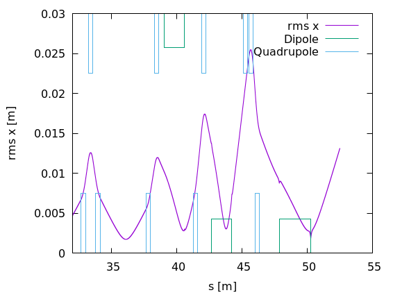
In the example below this file is used to indicate the positions of dipoles and quadrupoles in a plot of RMS x
plot '70MeV_Gantry2.stat' u 2:6 w l t 'rms x'
repl 'data/70MeV_Gantry2_ElementPositions.sdds' u 1:(-$2/0.45 + 1.6) w l axis x1y2 lc 2 t 'Dipole'
repl 'data/70MeV_Gantry2_ElementPositions.sdds' u 1:(-$2/0.45 - 1.6) w l axis x1y2 lc 2 notitle
repl 'data/70MeV_Gantry2_ElementPositions.sdds' u 1:(-$3 + 1.6) w l axis x1y2 lc 3 t 'Quadrupole'
repl 'data/70MeV_Gantry2_ElementPositions.sdds' u 1:(-$3 - 1.6) w l axis x1y2 lc 3 notitle
set xrange[32:]
set y2range[-1.2:1.2]
This produces a plot as found in 13
6.7.7. data/<input_file_name >_DesignPath.dat
The trajectory of the reference particle is stored in this ASCII file. The content of the columns are listed in the following table.
| Column Nr. | Name | Units | Meaning |
|---|---|---|---|
1 |
m |
Position in path length |
|
2 |
m |
X-component of position in floor coordinates |
|
3 |
m |
Y-component of position in floor coordinates |
|
4 |
m |
Z-component of position in floor coordinates |
|
5 |
1 |
X-component of momentum in floor coordinates |
|
6 |
1 |
Y-component of momentum in floor coordinates |
|
7 |
1 |
Z-component of momentum in floor coordinates |
|
8 |
MV m^-1 |
X-component of electric field at position |
|
9 |
MV m^-1 |
Y-component of electric field at position |
|
10 |
MV m^-1 |
Z-component of electric field at position |
|
11 |
T |
X-component of magnetic field at position |
|
12 |
T |
Y-component of magnetic field at position |
|
13 |
T |
Z-component of magnetic field at position |
|
14 |
MeV |
Kinetic energy |
|
15 |
s |
Time |
6.8. Multiple Species
In the present version only one particle species can be defined see Chapter Beam Command, however due to the underlying general structure, the implementation of a true multi species version of OPAL should be simple to accomplish.
6.9. Multipoles in different Coordinate systems
In the following sections there are three models presented for the fringe field of a multipole. The first one deals with a straight multipole, while the second one treats a curved multipole, both starting with a power expansion for the magnetic field. The last model tries to be different by starting with a more compact functional form of the field which is then adapted to straight and curved geometries.
6.9.1. Fringe field models
(for a straight multipole)
Most accelerator modeling codes use the hard-edge model for magnets - constant Hamiltonian. Real magnets always have a smooth transition at the edges - fringe fields. To obtain a multipole description of a field we can apply the theory of analytic functions.
Assuming that \(A\) has only a non-zero component \(A_s\) we get
These equations are just the Cauchy-Riemann conditions for an analytic function \(\tilde{A} (z) = A_s (x, y) + i V(x,y)\). So the complex potential is an analytic function and can be expanded as a power series
with \(\lambda_n, \mu_n\) being real constants. It is practical to express the field in cylindrical coordinates \((r, \varphi, s)\)
From the real and imaginary parts of equation () we obtain
Taking the gradient of \(-V(r, \varphi)\) we obtain the multipole expansion of the azimuthal and radial field components, respectively
Furthermore, we introduce the normal multipole coefficient \(b_n\) and skew coefficient \(a_n\) defined with the reference radius \(r_0\) and the magnitude of the field at this radius \(B_0\) (these coefficients can be a function of s in a more general case as it is presented further on).
To obtain a model for the fringe field of a straight multipole, a proposed starting solution for a non-skew magnetic field is
It is straightforward to derive a relation between coefficients
By identifying the term in front of the same powers of \(r\) we obtain the recurrence relation
The solution of the recursion relation becomes
Therefore
The transverse components of the field are
where the following gradients determine the entire potential and can be deduced from the function \(C_{n,0}(z)\) once the harmonic \(n\) is fixed.
The z-directed component of the filed can be expressed in a similar form
The gradient functions \(g_{rn}, g_{\varphi n}, g_{zn}\) are obtained from
One preferred model to approximate the gradient profile on the central axis is the k-parameter Enge function
where \(d(z)\) is the distance to the field boundary and \(\lambda\) characterizes the fringe field length.
6.9.2. Fringe field of a curved multipole
(fixed radius)
We consider the Frenet-Serret coordinate system \( ( \hat{\mathbf{x}}, \hat{\mathbf{s}}, \hat{\mathbf{z}} )\) with the radius of curvature \( \rho \) constant and the scale factor \( h_s = 1 + x/ \rho\). A conversion to these coordinates implies that
To simplify the problem, consider multipoles with mid-plane symmetry, i.e.
The most general form of the expansion is
Maxwell’s equations \( \nabla \cdot \mathbf{B} = 0 \) and \( \nabla \times \mathbf{B} = 0 \) in the above coordinates yield
The substitution of General form into Maxwell’s equations allows for the derivation of recursion relations. Maxwell equations gives
Equating the powers in \(x^i z^{2k}\)
A similar result is obtained from Maxwell equations
The last equation from \(\nabla \times \mathbf{B} = 0\) should be consistent with the two recursion relations obtained. Maxwell equations implies
This results follows directly from a factors and c factors; therefore the relations are consistent. Furthermore, the last required relations is obtained from the divergence of B
Using the relation (a factors) to replace the \(a\) coefficients with \(b\)’s we arrive at
All the coefficients above can be determined recursively provided the field \(B_z\) can be measured at the mid-plane in the form
where \(B_{i,0}\) are functions of \(s\) and they can model the fringe field for each multipole term \(x^n\). As an example, for a dipole magnet, the \(B_{1,0}\) function can be model as an Enge function or \(tanh\).
6.9.3. Fringe field of a curved multipole
(variable radius of curvature)
The difference between this case and the above is that \(\rho\) is now a function of \(s\), \(\rho(s)\). We can obtain the same result starting with the same functional forms for the field (General form). The result of the previous section also holds in this case since no derivative \(\frac{\partial}{\partial s}\) is applied to the scale factor \(h_s\). If the radius of curvature is set to be proportional to the dipole filed observed by some reference particle that stays in the centre of the dipole
6.9.4. Fringe field of a multipole
This is a different, more compact treatment The derivation is more clear if we gather the variables together in functions. We assume again mid-plane symmetry and that the z-component of the field in the mid-plane has the form
where \(T(s)\) is the transverse field profile and \(S(s)\) is the fringe field. One of the requirements of the symmetry is that \(B_z(z) = B_z(-z)\) which using a scalar potential \(\psi\) requires \(\frac{\partial \psi}{\partial z}\) to be an even function in z. Therefore, \(\psi\) is an odd function in z and can be written as
The given transverse profile requires that \(f_0(x,s) = T(x)S(s)\), while \(\nabla^2 \psi = 0\) follows from Maxwell’s equations as usual, more explicitly
For a straight multipole \(h_s = 1\). Laplace’s equation becomes
By equating powers of \(z\) we obtain the recursion relation
The general expression for any \(f_n(x,s)\) is then obtained from the mid-plane field by
For a curved multipole of constant radius \(h_s = 1 + \frac{x}{\rho} \quad \text{with} \quad \rho = const.\) The corresponding Laplace’s equation is
Again we substitute with the functional form of the potential to get the recursion
Finally consider what changes for \(\rho = \rho (s)\). Laplace’s equation is
The last step is again the substitution to get
If the radius of curvature is proportional to the dipole field in the centre of the multipole (the dipole component of the transverse field is a constant \(T_{dipole}(x) = B_0\) and
This expression can be replaced in ([eq.40]) to obtain a more explicit equation.
6.10. References
[7] J. Qiang et al., A three-dimensional quasi-static model for high brightness beam dynamics simulation, Tech. Rep. LBNL-59098, Lawrence Berkeley National Laboratory (2005).
[8] J. Qiang et al., Three-dimensional quasi-static model for high brightness beam dynamics simulation, Phys. Rev. ST Accel. Beams 9, 044204 (2006).
[9] J. Qiang et al., Erratum: three-dimensional quasi-static model for high brightness beam dynamics simulation, Phys. Rev. ST Accel. Beams 10, 12990 (2007).
[10] G. Fubaiani et al., Space charge modeling of dense electron beams with large energy spreads, Phys. Rev. ST Accel. Beams 9, 064402 (2006).
[11] C.K. Birdsall and A.B Langdon, Plasma physics via computer simulation (McGraw-Hill, New York, 1985).
[13] M. Borland, A self-describing file protocol for simulation integration and shared postprocessors, in Proceedings of the Particle Accelerator Conference (PAC'95), vol. 4, pp. 2184–2186 (Dallas, TX, USA, 1995).
[14] M. Borland et al., User’s guide for SDDS toolkit version 2.8.
[15] U. Ayachit, The ParaView Guide: A Parallel Visualization Application (Kitware, 2015).
7. OPAL-cycl
7.1. Introduction
OPAL-cycl, as one of the flavors of the OPAL framework, is a fully three-dimensional parallel beam dynamics simulation program dedicated to future high intensity cyclotrons and FFAs. It tracks multiple particles which takes into account the space charge effects. For the first time in the cyclotron community, OPAL-cycl has the capability of tracking multiple bunches simultaneously and take into account the beam-beam effects of the radially neighboring bunches (we call it neighboring bunch effects for short) by using a self-consistent numerical simulation model.
Apart from the multi-particle simulation mode, OPAL-cycl also has two other serial tracking modes for conventional cyclotron machine design. One mode is the single particle tracking mode, which is a useful tool for the preliminary design of a new cyclotron. It allows one to compute basic parameters, such as reference orbit, phase shift history, stable region, and matching phase ellipse. The other one is the tune calculation mode, which can be used to compute the betatron oscillation frequency. This is useful for evaluating the focusing characteristics of a given magnetic field map.
In addition, the widely used plugin elements, including collimator, radial profile probe, septum, trim-coil field and charge stripper, are currently implemented in OPAL-cycl. These functionalities are very useful for designing, commissioning and upgrading of cyclotrons and FFAs.
7.2. Tracking modes
According to the number of particles defined by the argument NPART in
BEAM (see Chapter Beam Command),
OPAL-cycl works in one of the following three operation modes automatically.
7.2.1. Single Particle Tracking mode
In this mode, only one particle is tracked, either with acceleration or not. Working in this mode, OPAL-cycl can be used as a tool during the preliminary design phase of a cyclotron.
The 6D parameters of a single particle in the initial local frame must
be read from a file. To do this, in the OPAL input file, the command
line DISTRIBUTION (see Chapter Distribution)
should be defined like this:
Dist1: DISTRIBUTION, TYPE=fromfile, FNAME="PartDatabase.dat";
where the file PartDatabase.dat should have two lines:
 1
 0.001 0.001   0.001   0.001   0.001  0.001
The number in the first line is the total number of particles. In the second line the data represents \(x, p_x, y, p_y, z, p_z\) in the local reference frame. Their units are described in Units.
Please don’t try to run this mode in parallel environment. You should believe that a single processor of the \(21^{st}\) century is capable of doing the single particle tracking.
7.2.2. Tune Calculation mode
In this mode, two particles are tracked, one with all data is set to zero is the reference particle and another one is an off-centering particle which is off-centered in both \(r\) and \(z\) directions. Working in this mode, OPAL-cycl can calculate the betatron oscillation frequency \(\nu_r\) and \(\nu_z\) for different energies to evaluate the focusing characteristics for a given magnetic field.
Like the single particle tracking mode, the initial 6D parameters of the two particles in the local reference frame must be read from a file, too. In the file should has three lines:
 2
 0.0   0.0   0.0   0.0   0.0   0.0
 0.001 0.0   0.0   0.0   0.001  0.0
When the total particle number equals 2, this mode is triggered
automatically. Only the element CYCLOTRON in the beam line is used and
other elements are omitted if any exists.
Please don’t try to run this mode in parallel environment, either.
7.2.3. Multi-particle tracking mode
In this mode, large scale particles can be tracked simultaneously, either with space charge or not, either single bunch or multi-bunch, either serial or parallel environment, either reading the initial distribution from a file or generating a typical distribution, either running from the beginning or restarting from the last step of a former simulation.
Because this is the main mode as well as the key part of OPAL-cycl, we will describe this in detail in Multi-bunch Mode.
7.3. Variables in OPAL-cycl
OPAL-cycl uses the following canonical variables to describe the motion of particles:
- X
-
Horizontal position \(x\) of a particle in given global Cartesian coordinates [m].
- PX
-
Horizontal canonical momentum [Units].
- Y
-
Longitudinal position \(y\) of a particle in global Cartesian coordinates [m].
- PY
-
Longitudinal canonical momentum [Units].
- Z
-
Vertical position \(z\) of a particle in global Cartesian coordinates [m].
- PZ
-
Vertical canonical momentum [Units].
The independent variable is: t [s].
7.3.1. The initial distribution in the local reference frame
The initial distribution of the bunch, either read from file or
generated by a distribution generator (see Chapter Distribution),
is specified in the local reference frame of the OPAL-cycl Cartesian
coordinate system (see Variables in OPAL-cycl). At the beginning of the
run, the 6 phase space variables \((x, y, z, p_x, p_y, p_z)\)
are transformed to the global Cartesian coordinates \((X, Y, Z, PX, PY, PZ)\) using the starting
coordinates \(r_0\) (RINIT), \(\phi_0\)
(PHIINIT), and \(z_0\) (ZINIT), and the starting momenta
\(p_{total}\) (defined by the beam energy specified in the Beam Command),
\(p_{r0}\) (PRINIT), and \(p_{z0}\) (PZINIT) of
the reference particle, defined in the CYCLOTRON
element. Note that \(p_{\phi 0}\) is calculated automatically from
\(p_{total}\), \(p_{r0}\), and \(p_{z0}\).
7.4. Field Maps
In OPAL-cycl, the magnetic field on the median plane is read from an ASCII type file. The field data should be stored in the cylinder coordinates frame (because the field map on the median plane of the cyclotron is usually measured in this frame).
With respect to the external magnetic field map two possible situations can be considered: in the first situation, the measured field map data is loaded by the tracker. In most cases, only the vertical field, \(B_z\), can be measured on the median plane (\(z=0\)). by using measurement equipment. Since the magnetic field outside the median plane is required to compute trajectories with \(z \neq 0\), the field needs to be expanded in the \(z\) direction. According to the approach given by Gordon and Taivassalo [18] by using a magnetic potential and measured \(B_z\) on the median plane at the point \((r,\theta, z)\) in cylindrical polar coordinates, the third order field can be written as:
where \(B_z\equiv B_z(r, \theta, 0)\) and
All the partial differential coefficients are computed from the median plane data by interpolation using Lagrange’s 5-point formula.
In the other situation, 3D magnetic field data for the region of interest is calculated numerically by building a 3D model using commercial software, such as TOSCA, ANSOFT and ANSYS during the design phase of a new cyclotron. If the field on the median plane is calculated, the field off the median plane can be obtained using the same expansion approach as the measured field map as described above. In this case the calculated field will be more accurate, especially at large distances from the median plane i.e. a full 3D field map can be calculated.
In the current version, we implemented three specific type
field-read functions Cyclotron::getFieldFromFile() of the median plane
fields. Which function is used is controlled by the parameters
TYPE of CYCLOTRON in the input file.
7.4.1. CARBONCYCL type
If TYPE=CARBONCYCL, the program requires the \(B_z\) data
which is stored in a sequence shown in Figure 14.
We need to add 6 parameters at the header of a plain \(B_z\) [kG] data file, namely, \(r_{min}\) [mm], \(\Delta r\) [mm], \(\theta_{min}\) [\(^{\circ}\)], \(\Delta \theta\) [\(^{\circ}\)], \(N_\theta\) (total data number in each arc path of azimuthal direction) and \(N_r\) (total path number along radial direction). If \(\Delta r\) or \(\Delta \theta\) is decimal, one can set its negative opposite number. For instance, if \(\Delta \theta = \frac{1}{3}{^{\circ}}\), the fourth line of the header should be set to -3.0. Example showing the above explained format:
3.0e+03
10.0
0.0
-3.0
300
161
1.414e-03  3.743e-03  8.517e-03  1.221e-02  2.296e-02
3.884e-02  5.999e-02  8.580e-02  1.150e-01  1.461e-01
1.779e-01  2.090e-01  2.392e-01  2.682e-01  2.964e-01
3.245e-01  3.534e-01  3.843e-01  4.184e-01  4.573e-01
                        ...
The number of values per column is arbitrary.
7.4.2. CYCIAE type
If TYPE=CYCIAE, the program requires data format given by ANSYS10.0.
This function is originally for the 100 MeV cyclotron of CIAE, whose
isochronous fields is numerically computed by ANSYS. The median plane
fields data is output by reading the APDL (ANSYS Parametric Design
Language) script during the post-processing phase (you may need to do
minor changes to adapt your own cyclotron model):
/post1
resume,solu,db
csys,1
nsel,s,loc,x,0
nsel,r,loc,y,0
nsel,r,loc,z,0
PRNSOL,B,COMP

CSYS,1
rsys,1

*do,count,0,200
   path,cyc100_Ansys,2,5,45
   ppath,1,,0.01*count,0,,1
   ppath,2,,0.01*count/sqrt(2),0.01*count/sqrt(2),,1

   pdef,bz,b,z
   paget,data,table

   *if,count,eq,0,then
      /output,cyc100_ANSYS,dat
      *STATUS,data,,,5,5
      /output
   *else
      /output,cyc100_ANSYS,dat,,append
      *STATUS,data,,,5,5
      /output
   *endif
*enddo
finish
By running this in ANSYS, you can get a fields file with the name cyc100_ANSYS.data. You need to put 6 parameters at the header of the file, namely, \(r_{min}\) [mm], \(\Delta r\) [mm], \(\theta_{min}\) [\(^{\circ}\)], \(\Delta \theta\) [\(^{\circ}\)], \(N_\theta\)(total data number in each arc path of azimuthal direction) and \(N_r\)(total path number along radial direction). If \(\Delta r\) or \(\Delta \theta\) is decimal, one can set its negative opposite number. This is useful if the decimal is unlimited. For instance, if \(\Delta \theta = \frac{1}{3} {^{\circ}}\), the fourth line of the header should be -3.0. In other words, the fields are stored in the following format:
0.0
10.0
0.0e+00
1.0e+00
90
201
 PARAMETER STATUS- DATA  ( 336 PARAMETERS DEFINED)
                  (INCLUDING    17 INTERNAL PARAMETERS)

      LOCATION                VALUE
        1       5       1   0.537657876
        2       5       1   0.538079473
        3       5       1   0.539086731
                  ...
       44       5       1   0.760777286
       45       5       1   0.760918663
       46       5       1   0.760969074

 PARAMETER STATUS- DATA  ( 336 PARAMETERS DEFINED)
                  (INCLUDING    17 INTERNAL PARAMETERS)

      LOCATION                VALUE
        1       5       1   0.704927299
        2       5       1   0.705050993
        3       5       1   0.705341275
                  ...
7.4.3. BANDRF type
BANDRF fieldmap TYPE allows to read both the magnetic field and the
electric field from the CYCLOTRON
element. The magnetic field data (\(B_z\)) are stored in the same
format as CARBONCYCL. Regarding
the electric field, the 3D RF field-map can be read from H5Hut
type file (.h5part file extension) making use of a conversion tool integrated
into OPAL: ascii2h5block. For the details about its usage, please see
Read 3D RF field-map.
The electric field map can be imported from some field files, which can be
optionally superposed, providing different meshing specifications for the
field map. This is useful for modeling the central region electric fields
which usually has complicated shapes. Please note that in this case, the E
field is treated as a part of CYCLOTRON element, rather than an independent
RFCAVITY element.
7.4.4. RING type
If TYPE=RING, the program requires the data format like PSI format field file
ZYKL9Z.NAR and SO3AV.NAR, which was given by the measurement. We add
4 parameters at the header of the file, namely, \(r_{min}\) [mm],
\(\Delta r\) [mm], \(\theta_{min}\)[\(^{\circ}\)],
\(\Delta \theta\)[\(^{\circ}\)]. If \(\Delta r\) or
\(\Delta \theta\) is decimal, one can set its negative opposite
number. This is useful if the decimal is unlimited. For instance, if
\(\Delta \theta = \frac{1}{3}{^{\circ}}\), the fourth line of
the header should be -3.0.
1900.0
20.0
0.0
-3.0
 LABEL=S03AV
 CFELD=FIELD     NREC=  141      NPAR=    3
 LPAR=    7      IENT=    1      IPAR=    1
               3             141             135              30               8
               8              70
 LPAR= 1089      IENT=    2      IPAR=    2
 0.100000000E+01 0.190000000E+04 0.200000000E+02 0.000000000E+00 0.333333343E+00
 0.506500015E+02 0.600000000E+01 0.938255981E+03 0.100000000E+01 0.240956593E+01
 0.282477260E+01 0.340503168E+01 0.419502926E+01 0.505867147E+01 0.550443363E+01
 0.570645094E+01 0.579413509E+01 0.583940887E+01 0.586580372E+01 0.588523722E+01
                        ...
7.4.5. 3D field-map
It is additionally possible to load 3D field-maps for tracking through
OPAL-cycl. 3D field-maps are loaded by sequentially adding new field
elements to a line, as is done in OPAL-t. It is not possible to add RF
cavities while operating in this mode. In order to define ring
parameters such as initial ring radius a RINGDEFINITION type is loaded
into the line, followed by one or more SBEND3D elements.
ringdef: RINGDEFINITION, HARMONIC_NUMBER=6, LAT_RINIT=2350.0, LAT_PHIINIT=0.0,
         LAT_THETAINIT=0.0, BEAM_PHIINIT=0.0, BEAM_PRINIT=0.0,
         BEAM_RINIT=2266.0, SYMMETRY=4.0, RFFREQ=0.2;

triplet: SBEND3D, FMAPFN="fdf-tosca-field-map.table", LENGTH_UNITS=10., FIELD_UNITS=-1e-4;

l1: Line = (ringdef, triplet, triplet);
The field-map with file name fdf-tosca-field-map.table is loaded, which is a file like
      422280      422280      422280           1
 1 X [LENGU]
 2 Y [LENGU]
 3 Z [LENGU]
 4 BX [FLUXU]
 5 BY [FLUXU]
 6 BZ [FLUXU]
 0
 194.01470 0.0000000 80.363520 0.68275932346E-07 -5.3752492577 0.28280706805E-07
 194.36351 0.0000000 79.516210 0.42525693524E-07 -5.3827955117 0.17681348191E-07
 194.70861 0.0000000 78.667380 0.19766168358E-07 -5.4350026348 0.82540823165E-08
<continues>
The header parameters are ignored - user supplied parameters
LENGTH_UNITS and FIELD_UNITS are used. Fields are supplied on points
in a grid in \((r, y, \phi)\). Positions and field elements
are specified by Cartesian coordinates \((x, y, z)\).
7.4.6. User’s own field-map
You should revise the function or write your own function according to
the instructions in the code to match your own field format if it is
different to above types. For more detail about the parameters of
CYCLOTRON, please refer to Cyclotron.
7.5. RF field
7.5.1. Read RF voltage profile
The RF cavities are treated as straight lines with infinitely narrow gaps and the electric field is a \(\delta\) function plus a transit time correction. The two-gap cavity is treated as two independent single-gap cavities. The spiral gap cavity is not implemented yet. For more detail about the parameters of cyclotron cavities, see Cyclotron.
The voltage profile of a cavity gap is read from ASCII file. Here is an example:
6
0.00      0.15      2.40
0.20      0.65      2.41
0.40      0.98      0.66
0.60      0.88     -1.59
0.80      0.43     -2.65
1.00     -0.05     -1.71
The number in the first line means 6 sample points and in the following lines the three values represent the normalized distance to the inner edge of the cavity, the normalized voltage and its derivative respectively.
7.5.2. Read 3D RF field-map
The 3D RF field-map can be read from H5Hut type file for
TYPE=BANDRF. To generate the h5part field files, it is necessary to use the
ascii2h5block conversion tool. This program builds h5part field files from
ASCII file output of ANSYS or OPERA 3D field data. The command to use it should be like:
ascii2h5block efield.txt hfield.txt ehfout
The ASCII input files must be adapted for an adequate conversion. The first three rows of a field map that you wish to combine should include integers with the amount of steps (or different values) in \(x\), \(y\) and \(z\). The 2D mid-plane map is in cylindrical coordinates, while the 3D map must be in Cartesian coordinates.
7.6. Particle Tracking and Acceleration
The precision of the tracking methods is vital for the entire simulation process, especially for long distance tracking jobs. OPAL-cycl uses a fourth order Runge-Kutta algorithm and the second order Leap-Frog scheme. The fourth order Runge-Kutta algorithm needs four external magnetic field evaluations in each time step \(\tau\). During the field interpolation process, for an arbitrary given point the code first interpolates Formula \(B_z\) for its counterpart on the median plane and then expands to this given point using [eq-Bfield].
After each time step \(i\), the code detects whether the particle crosses any one of the RF cavities during this step. If it does, the time point \(t_c\) of crossing is calculated and the particle return back to the start point of step \(i\). Then this step is divided into three sub-steps: first, the code tracks this particle for \( t_1 = \tau - (t_c-t_{i-1})\); then it calculates the voltage and adds momentum kick to the particle and refreshes its relativistic parameters \(\beta\) and \(\gamma\); and then tracks it for \(t_2 = \tau - t_1\).
7.7. Space Charge
OPAL-cycl uses the same solvers as OPAL-t to calculate the space charge effects see Chapter Field Solver.
Typically, the space charge field is calculated once per time step. This is no surprise for the second order Boris-Buneman time integrator (leapfrog-like scheme) which has per default only one force evaluation per step. The fourth order Runge-Kutta integrator keeps the space charge field constant for one step, although there are four external field evaluations. There is an experimental multiple-time-stepping (MTS) variant of the Boris-Buneman/leapfrog-method, which evaluates space charge only every N^th step, thus greatly reducing computation time while usually being still accurate enough.
7.8. Multi-bunch Mode
The neighboring bunches problem is motivated by the fact that for high intensity cyclotrons with small turn separation, single bunch space charge effects are not the only contribution. Along with the increment of beam current, the mutual interaction of neighboring bunches in radial direction becomes more and more important, especially at large radius where the distances between neighboring bunches get increasingly small and even they can overlap each other. One good example is PSI 590 MeV Ring cyclotron with a current of about 2 mA in CW operation and the beam power amounts to 1.2 MW. An upgrade project for Ring is in process with the goal of 1.8 MW CW on target by replacing four old aluminum resonators by four new copper cavities with peak voltage increasing from about 0.7 MW to above 0.9 MW. After upgrade, the total turn number is reduced from 200 turns to less than 170 turns. Turn separation is increased a little bit, but still are at the same order of magnitude as the radial size of the bunches. Hence once the beam current increases from 2 mA to 3 mA, the mutual space charge effects between radially neighboring bunches can have significant impact on beam dynamics. In consequence, it is important to cover neighboring bunch effects in the simulation to quantitatively study its impact on the beam dynamics.
In OPAL-cycl, we developed a new fully consistent algorithm of
multi-bunch simulation. We implemented two working modes, namely ,
AUTO and FORCE. In the first mode, only a single bunch is tracked
and accelerated at the beginning, until the radial neighboring bunch
effects become an important factor to the bunches’ behavior. Then the
new bunches will be injected automatically to take these effects into
account. In this way, we can save time and memory, and more important,
we can get higher precision for the simulation in the region where
neighboring bunch effects are important. In the other mode, multi-bunch
simulation starts from the injection points.
In the space charge calculation for multi-bunch, the computation region covers all bunches. Because the energy of the bunches is quite different, it is inappropriate to use only one particle rest frame and a single Lorentz transformation any more. So the particles are grouped into different energy bins and in each bin the energy spread is relatively small. We apply Lorentz transforming, calculate the space charge fields and apply the back Lorentz transforming for each bin separately. Then add the field data together. Each particle has a ID number to identify which energy bin it belongs to.
7.9. Input
All the three working modes of OPAL-cycl use an input file written in
mad language which will be described in detail in the following
chapters.
For the Tune Calculation mode, one additional auxiliary file with the following format is needed.
   72.000 2131.4   -0.240
   74.000 2155.1   -0.296
   76.000 2179.7   -0.319
   78.000 2204.7   -0.309
   80.000 2229.6   -0.264
   82.000 2254.0   -0.166
   84.000 2278.0    0.025
In each line the three values represent energy \(E\), radius \(r\) and \(P_r\) for the SEO (Static Equilibrium Orbit) at starting point respectively and their units are MeV, mm and mrad.
A bash script tuning.sh is shown on the next page, to execute OPAL-cycl for tune calculations.
To start execution, just run tuning.sh which uses the input file testcycl.in and the auxiliary file FIXPO SEO_. The output file is plotdata from which one can plot the tune diagram.
7.10. Output
OPAL-cycl writes out several output files, some specific to the Tracking mode (see following sections).
7.10.1. <input_file_name >.stat
See OPAL-t stat file. The only difference is in the cyclotron coordinate convention. The z (or s) coordinate refers to the vertical direction and y corresponds to the longitudinal or beam travel direction.
7.10.2. Single Particle Tracking mode
The intermediate phase space data is stored in an ASCII file which can
be used to plot the orbit. The file’s name is combined by input file
name (without extension) and -trackOrbit.dat. The data are stored in
the global Cartesian coordinates. The frequency of the data output can
be set using the option SPTDUMPFREQ of OPTION statement.
The phase space data per STEPSPERTURN (a parameter in the TRACK
command) steps is stored in an ASCII file. The file’s is named
<input_file_name >-afterEachTurn.dat. The data is stored in the global cylindrical
coordinate system. Please note that if the field map is ideally
isochronous, the reference particle of a given energy take exactly one
revolution in STEPSPERTURN steps; Otherwise, the particle may not go
through a full 360\(^{\circ}\) in STEPSPERTURN steps.
There are 3 ASCII files which store the phase space data around \(0\), \(\pi/8\) and \(\pi/4\) azimuths. Their names are the combinations of input file name (without extension) and -Angle0.dat, -Angle1.dat and -Angle2.dat respectively. The data is stored in the global cylindrical coordinate system, which can be used to check the property of the closed orbit.
7.10.3. Tune calculation mode
The tunes \(\nu_r\) and \(\nu_z\) of each energy are stored in a ASCII file named tuningresult.
7.10.4. Multi-particle tracking mode
The intermediate phase space data of all particles and some interesting
parameters, including RMS envelop size, RMS emittance, external field,
time, energy, length of path, number of bunches and tracking step, are
stored in the H5hut file-format [19] and can be analyzed
using H5root [20], [21]. The frequency of the data output can
be set using the PSDUMPFREQ option of OPTION statement.
The file is named <input_file_name >.h5.
This output can be switched on or off with the option ENABLEHDF5.
The intermediate phase space data of central particle (with ID of 0) and
an off-centering particle (with ID of 1) are stored in an ASCII file.
The file is named <input_file_name >-trackOrbit.dat.
The frequency of the data output can be set using
the SPTDUMPFREQ option of OPTION statement.
7.10.5. Field maps
The magnetic field map read by OPAL could be saved into an output file called
gnu.out. This file stores the magnetic field \(B_z\) data in the
median plane in cylindrical coordinates following the sequence shown in
Figure 14. This output file is available in the cyclotron field types
CARBONCYCL, BANDRF, FFA and AVFEQ.
In case of CARBONCYCL or BANDRF an additional output field file an
additional output field file is saved (eb.out), storing three vectors with
the position, electric field and the magnetic field.
Writing these output files is enabled when OPAL is run on single node, and
it can be switched on or off with the INFO option of
OPTION statement.
Moreover, DUMPFIELDS and DUMPEMFIELDS routines (see Chapter Field Output)
can be employed to write out the external field used in OPAL-cycl in a
different grid than the input field maps.
7.11. Matched Distribution
In order to run matched distribution simulation one has to specify a periodic accelerator. The function call also needs the symmetry of the machine as well as a field map. The user then specifies the emittance \(\pi\) \(mm\) \(mrad\).
/*
 * specify periodic accelerator
 */
l1 = ...

/*
 * try finding a matched distribution
 */
Dist1:DISTRIBUTION, TYPE=GAUSSMATCHED, LINE=l1, FMAPFN=...,
                    MAGSYM=..., EX = ..., EY = ..., ET = ...;
7.11.1. Example
Simulation of the PSI Ring Cyclotron at 580 MeV and current 2.2 mA. The
program finds a matched distribution followed by a bunch initialization
according to the matched covariance matrix.
The matched distribution algorithm works with normalized emittances,
i.e. normalized by the lowest energy of the machine. The printed
emittances, however, are the geometric emittances. In addition, it has
to be paid attention that the computation is based on
\((x,x',y,y',z,\delta)\) instead of
\((x,p_{x},y,p_{y},z,p_{z})\). Since the particles are
represented in the latter coordinate system, the corresponding
transformation has to be applied to obtain the rms emittances that are
given in the output.
Input file
All supplementary files can be found in the matched distribution regression test.
Output
7.12. References
[18] M. M. Gordon and V. Taivassalo, Nonlinear Effects of Focusing Bars Used in the Extraction Systems of Superconducting Cyclotrons, IEEE Trans. Nucl. Sci. 32, 2447 (1985)
[19] M. Howison et al., H5hut: A High-Performance I/O Library for Particle-based Simulations, in 2010 IEEE International Conference on Cluster Computing Workshops and Posters, vol. 1, pp. 1–8 (Heraklion, Crete, 2010)
[21] T. Schietinger, H5PartROOT - A visualization and post-processing tool for accelerator simulations, in Proceedings of the 10th International Computational Accelerator Physics conference (ICAP09), pp. 343-346 (San Francisco, CA, USA, 2009)
8. OPAL-map
8.1. Introduction
OPAL-map is a map tracking beam optics code. This type computes maps for each beam line element to describe the action of the system.
The map creation is done by applying the Lie Operator on the element Hamiltonian and calculated in the Truncated Power Series Algebra (TPSA)[22]. The TPSA is a Differential Algebra (DA), which uses the Taylor expansion as the equivalent function. In OPAL-map the TPSA gets provided from the own OPAL DA package.
In contrast to time \(t\) dependent tracking codes, as OPAL-t, map tracking codes use the longitudinal bunch position \(s\) as independent variable. Furthermore, map tracking codes do not use numerical integrators for the determination of the particle trajectory, which can be a computationally very expensive.
The main advantage in map tracking codes lies in the ''map'' itself. These do not only contain valuable information about the beam line, but also can be accumulated to reduce the computational effort in the particle tracking.
8.2. Variables in OPAL-map
For in and outputs, the units as in Variables in OPAL-t are used.
OPAL-map uses an Frenet-Serret coordinate system, referring on a reference particle. This particle has the ideal properties, ergo follows the design path. The following canonical variables to describe the motion of particles. The physical units are listed in square brackets.
- X
-
Horizontal position \(x\) of a particle relative to the reference particle [m].
- PX
-
\(\frac{p_x}{P_0}\) Normalized horizontal canonical momentum [1]. (Where \(p_x\) is the momentum of the particle and \(P_0\) is the momentum of the reference particle)
- Y
-
Vertical position \(y\) of a particle relative to the reference particle [m].
- PY
-
\(\frac{p_y}{P_0}\) Normalized vertical canonical momentum [1].
- Z
-
Longitudinal position \(z\) of a particle relative to the reference particle [m].
- DELTA
-
\(\frac{E}{P_0 c}-\frac{1}{\beta_0}\) Energy derivation [1]. (Where \(E\) is the total energy of the particle and \(\beta_0 = \frac{u}{c}\) the speed relative to the speed of light \(c\) of the reference particle)
The independent variable is position of the reference particle s [m].
8.3. Principle of Map Tracking
The particle motion gets calculated by applying the map on the particle parameter.
Where \(v\) denotes the final (\(v^f\)) and initial (\(v^i\)) six dimensional phase space vector of each particle. \(\mathbf{\mathcal{M}}\) is the map. This map can represent either a beam element slice, the whole element, a beam line section or the whole system.
8.3.1. Creation of map
The creation of the element map is based on the Hamiltonian Mechanic, more specifically on the Lie Operator.
Here \(H\), the time dependent Hamiltonian represents the total energy, consisting of the kinetic \(T\) and potential \(V\) energy. The lower equations are the Hamiltonian equations of motion, where the momenta \(p_i\) and the positions \(q_i\) form the canonical pairs. Using canonical transformations, the Hamiltonian can be adjusted to use the path length \(s\) as independent and the particle parameters as dependent variable(s).
Introducing the Lie operator, which acts similar to a "waiting" Poisson Bracket:
If a function \(f:= f \left( \mathbf{q_{(s)}},\mathbf{p_{(s)}}\right) \) describes one of the phase space variables \(v\) its total derivative to the independent variable, combined with the Hamiltonian equations of motions, is similar to the Lie operator times the indepedent variable, i. e. \(s\).
The integral over the independent variable \(\int \cdot ds\):
Where \(e^{-:\!H\!: s}\) is the Lie expansion.
8.3.2. Implementation of map tracking
For the derivative of the Hamiltonian, a Differential Algebra (DA) was used, in particular the Truncated Power Series Algebra (TPSA). This algebra uses the Taylor expansion as the equivalent function, which also is responsible for its name by creating truncated power series. Just form the definition of the Taylor expansion, it can be seen that a finite, to the order \(\Omega\), expansion is an approximation of the actual function, due to the error term \(\mathcal{O}\left( \mathbf{v}^{\,\Omega +1}\left( \Delta s\right)\right) \).
In OPAL-map the Hamiltonian gets Taylor expanded and its map derived (Creation of Map) in the TPSA using the OPAL DA package. The truncation length gets defined in TRACK setting the MAP_ORDER attribute.
TRACK, LINE= QUADTEST, BEAM=BEAM1, MAXSTEPS=10000, DT=1.0e-10, ZSTOP=4.0, MAP_ORDER=2;
8.4. Additional Parameter in OPAL-map
| Attribute Name | set in | Default Value | Units | Description |
|---|---|---|---|---|
|
|
|
[ ] |
defines the map order ( = order TPSA - 1). |
|
beam line element |
|
[ ] |
defines the number of steps inside the element. |
8.4.1. Limitations
OPAL-map is the new flavour of OPAL and currently just contains the fundamental beam line elements:
-
Drift (
Drift), -
Dipole (
Sbend), -
Quadrupole (
Quadrupole)
8.5. Example
FODO lattice: MAP-FODO.in
Input distribution (to be put in directory data): FODO_DIST.dat
To RUN OPAL-map, the METHOD attribute gets set to THICK.
RUN, METHOD = "THICK", BEAM=BEAM1, FIELDSOLVER=FS1, DISTRIBUTION=DIST1;
The maximal order of the beam line maps get defined with the MAP_ORDER attribute.
TRACK, LINE= QUADTEST, BEAM=BEAM1, MAXSTEPS=10000, DT=1.0e-10, ZSTOP=4.0, MAP_ORDER=2;
As an optional parameter for the beam line elements NSlices=<x> provides the opportunity to split one element in <x> smaller steps. Otherwise, the default value is defined with 1.
D1:  DRIFT,             L=1.,                ELEMEDGE=0.000, NSLICES=10;
QP1: QUADRUPOLE,        L=0.3,  K1= 8.64195, ELEMEDGE=1.000, NSLICES=15;
8.6. Output
In addition to the progress report that OPAL-map writes to the standard output (stdout) it also writes different files for various purposes.
8.6.1. <input_file_name >.stat
The file structure is analogous to OPAL-t .stat file.
8.6.2. data/<input_file_name >.dispersion
OPAL-map computes the dispersion of the beam line according to:
where \(R\) is the Transfermatrix and \(\eta\) is the dispersion.
| Column Nr. | Name | Units | Meaning |
|---|---|---|---|
1 |
position |
m |
Longitudinal position |
2 |
\(\eta_x\) |
m |
Spatial dispersion in x |
3 |
\(\eta_{px}\) |
1 |
Momentum dispersion in x |
4 |
\(\eta_y\) |
m |
Spatial dispersion in x |
5 |
\(\eta_{py}\) |
1 |
Momentum dispersion in y positions |
8.6.3. data/<input_file_name >.map
Here the transfer map of the whole beamline gets printed.
Its format is analogous to a DA- FVPs (src/Classic/FixedAlgebra), where the polynomials (DA- FTPs) get represented in a 6 dimensional vector.
The first number describes the coefficient and the following 6 the variables of the monomial.
| Column Nr. | Name | Units | Meaning |
|---|---|---|---|
1 |
coefficient |
1 |
coefficient of monomial |
2 |
\(x\) |
1 |
\(x\) in monomial |
3 |
\(p_x\) |
1 |
\(p_x\) in monomial |
4 |
\(y\) |
1 |
\(y\) in monomial |
5 |
\(p_y\) |
1 |
\(p_y\) in monomial |
6 |
\(z\) |
1 |
\(z\) in monomial |
7 |
\(\delta\) |
1 |
\(\delta\) in monomial |
8.7. References
[22] M. Berz, Modern map methods in particle beam physics (Academic Press, San Diego, 1999)
9. Command Format
All flavors of OPAL using the same input language the MAD language. The language dialect here is ajar to MAD9, for hard core MAD8 users there is a conversion guide.
It is the first time that machines such as cyclotrons, proton and electron linacs can be described within the same language in the same simulation framework.
9.1. Statements and Comments
Input for OPAL is free format, and the line length is not limited.
During reading, input lines are normally printed on the echo file, but
this feature can be turned off for long input files. The input is broken
up into tokens (words, numbers, delimiters etc.), which form a sequence
of commands, also known as statements. Each statement must be terminated
by a semicolon (;), and long statements can be continued on any number
of input lines. White space, like blank lines, spaces, tabs, and
newlines are ignored between tokens. Comments can be introduced with two
slashes (//) and any characters following the slashes on the same line
are ignored.
The C convention for comments is also accepted. The comment delimiters can be nested; this allows to "comment out" sections of input.
In the following descriptions, words in lower case stand for syntactic
units which are to be replaced by actual text. UPPER CASE is used for
keywords or names. These must be entered as shown. Ellipses (…) are
used to indicate repetition.
The general format for a command is
keyword,attribute,...,attribute;
label:keyword,attribute,...,attribute;
It has three parts:
-
The
labelis required for a definition statement. Its must be an identifier see Identifiers or Labels and gives a name to the stored command. -
The
keywordidentifies the action desired. It must be an identifier see Identifiers or Labels. -
Each
attributeis entered in one of the formsattribute-name attribute-name=attribute-value attribute-name:=attribute-value
and serves to define data for the command, where:
-
The
attribute-nameselects the attribute, it must be an identifier see Identifiers or Labels. -
The
attribute-valuegives it a value see Command Attribute Types. When the attribute value is a constant or an expression preceded by the delimiter=it is evaluated immediately and the result is assigned to the attribute as a constant. When the attribute value is an expression preceded by the delimiter:=the expression is retained and re-evaluated whenever one of its operands changes.Each attribute has a fixed attribute type see Command Attribute Types.
Theattribute-valuecan only be left out for logical attributes, this implies atruevalue.
-
When a command has a label, OPAL keeps the command in memory. This
allows repeated execution of the same command by entering its label
only:
label;
or to re-execute the command with modified attributes:
label,attribute,...,attribute;
If the label of such a command appears together with new attributes, OPAL makes a copy of the stored command, replaces the attributes entered, and then executes the copy:
QF:QUADRUPOLE,L=1,K1=0.01; // first definition of QF
QF,L=2;                    // redefinition of QF

MATCH;
...
LMD:LMDIF,CALLS=10;           // first execution of LMD
LMD;                          // re-execute LMD with
                              // the same attributes
LMD,CALLS=100,TOLERANCE=1E-5; // re-execute LMD with
                              // new attributes
ENDMATCH;
9.2. Identifiers or Labels
An identifier refers to a keyword, an element, a beam line, a variable, an array, etc.
A label begins with a letter, followed by an arbitrary number of
letters, digits, periods (.), underscores (_). Other special
characters can be used in a label, but the label must then be enclosed
in single or double quotes. It makes no difference which type of quotes
is used, as long as the same are used at either end. The preferred form
is double quotes. The use of non-numeric characters is however strongly
discouraged, since it makes it difficult to subsequently process an
_OPAL_ output with another program.
When a name is not quoted, it is converted to upper case; the resulting name must be unique. An identifier can also be generated from a string expression see String Attributes.
9.3. Command Attribute Types
An object attribute is referred to by the syntax
object-name->attribute-name
If the attribute is an array see Arrays, one of its components is found by the syntax
object-name->attribute-name[index]
The following types of command attributes are available in OPAL:
String |
|
Logical |
|
Real expression |
|
Deferred expression |
|
Place |
|
Range |
|
Constraint |
|
Variable Reference |
|
Regular expression |
|
Array |
|
Array of logical |
|
Array of real |
|
Array of string |
|
Array of token lists |
See also:
Operators |
|
Functions |
|
Real functions of arrays |
|
Operand |
|
Random generators |
9.4. String Attributes
A string attribute makes alphanumeric information available, e.g. a
title, file name, element class name, or an option. It can contain any
characters, enclosed in single (’) or double (") quotes. However, if
it contains a quote, this character must be doubled. Strings can be
concatenated using the & operator see Table 5. An operand
in a string can also use the function STRING see Table 6.
String values can occur in string arrays see Arrays.
| Operator | Meaning | result type | operand types |
|---|---|---|---|
|
concatenate the strings |
string |
string,string |
| Function | Meaning | result type | argument type |
|---|---|---|---|
|
return string representation of the value of the numeric
expression |
string |
real |
Examples:
TITLE,"This is a title for the program run ""test""";
CALL,FILE="save";

REAL X=1;
STRING L2=LEP&STRING(X+1);
The second example converts the value of the expression X+1 to a
string and appends it to LEP, giving the string LEP2.
9.5. Logical Expressions
Many commands in OPAL require the setting of logical values (flags) to
represent the on/off state of an option. A logical value is represented
by one of the values TRUE or FALSE, or by a logical expression. A
logical expression can occur in logical arrays see Logical Arrays.
A logical expression has the same format and operator precedence as a logical expression in C. It is built from logical operators see Table 7 and logical operands:
relation      ::= "TRUE" |
                  "FALSE" |
                  real-expr rel-operator real-expr

rel-operator  ::= "==" | "!=" | "<" | ">" | ">=" | "<="

and-expr      ::= relation | and-expr "&&" relation

logical-expr  ::= and-expr | logical-expr "||" and-expr
| Operator | Meaning | result type | operand type |
|---|---|---|---|
|
true, if |
logical |
real,real |
|
true, if |
logical |
real,real |
|
true, if |
logical |
real,real |
|
true, if |
logical |
real,real |
|
true, if |
logical |
real,real |
|
true, if |
logical |
real,real |
|
true, if both |
logical |
logical,logical |
|
true, if at least one of |
logical |
logical,logical |
Example:
OPTION,ECHO=TRUE; // output echo is desired
When a logical attribute is not entered, its default value is always
FALSE. When only its name is entered, the value is set to TRUE:
OPTION,ECHO; // same as above
Example of a logical expression:
X>10 && Y<20 || Z==15
9.6. Real Expressions
To facilitate the definition of interdependent quantities, any real value can be entered as an arithmetic expression. When a value used in an expression is redefined by the user or changed in a matching process, the expression is re-evaluated. Expression definitions may be entered in any order. OPAL evaluates them in the correct order before it performs any computation. At evaluation time all operands used must have values assigned. A real expression can occur in real arrays see Real Arrays.
A real expression is built from operators see Table 8 and operands see Operands in Expressions:
real-ref  ::= real-variable |
              real-array "[" index "]" |
              object "->" real-attribute |
              object "->" real-array-attribute "[" index "]" |

table-ref ::= table "@" place "->" column-name

primary   ::= literal-constant |
              symbolic-constant |
              "#" |
              real-ref |
              table-ref |
              function-name "(" arguments ")" |
              (real-expression)

factor    ::= primary |
              factor "^" primary

term      ::= factor |
              term "*" factor |
              term "/" factor

real-expr ::= term |
              "+" term |
              "-" term |
              real-expr "+" term |
              real-expr "-" term |
It may contain functions see Table 9, Parentheses indicate operator precedence if required. Constant sub-expressions are evaluated immediately, and the result is stored as a constant.
9.7. Operators
An expression can be formed using operators see Table 8 and functions see Table 9 acting on operands see Operands in Expressions.
| Operator | Meaning | result type | operand type(s) |
|---|---|---|---|
Real operators with one operand |
|||
|
unary plus, returns |
real |
real |
|
unary minus, returns the negative of |
real |
real |
Real operators with two operands |
|||
|
add |
real |
real,real |
|
subtract |
real |
real,real |
|
multiply |
real |
real,real |
|
divide |
real |
real,real |
|
power, return |
real |
real,real |
| Function | Meaning | result type | argument type(s) |
|---|---|---|---|
Real functions with no arguments |
|||
|
random number, uniform distribution in [0,1) |
real |
- |
|
random number, Gaussian distribution with \(\mu=0\) and \(\sigma=1\) |
real |
- |
|
returns the kinetic energy of the bunch (MeV) |
real |
- |
|
random number, user-defined distribution |
real |
- |
Real functions with one argument |
|||
|
truncate |
real |
real |
|
round |
real |
real |
|
return largest integer not greater than |
real |
real |
|
return smallest integer not less than |
real |
real |
|
return sign of |
real |
real |
|
return square root of |
real |
real |
|
return natural logarithm of |
real |
real |
|
return exponential to the base \(e\) of |
real |
real |
|
return trigonometric sine of |
real |
real |
|
return trigonometric cosine of |
real |
real |
|
return absolute value of |
real |
real |
|
return trigonometric tangent of |
real |
real |
|
return inverse trigonometric sine of |
real |
real |
|
return inverse trigonometric cosine of |
real |
real |
|
return inverse trigonometric tangent of |
real |
real |
|
random number, Gaussian distribution with
\(\sigma\)=1, truncated at |
real |
real |
|
random number, user-defined distribution with one parameter |
real |
real |
|
evaluate the argument immediately and transmit it as a constant |
real |
real |
Real functions with two arguments |
|||
|
return inverse trigonometric tangent of |
real |
real,real |
|
return the larger of |
real |
real,real |
|
return the smaller of |
real |
real,real |
|
return the largest value less than |
real |
real,real |
|
random number, user-defined distribution with two parameters |
real |
real,real |
| Function | Meaning | result type | operand type |
|---|---|---|---|
|
return largest array component |
real |
real array |
|
return smallest array component |
real |
real array |
|
return rms value of an array |
real |
real array |
|
return absolute largest array component |
real |
real array |
Care must be used when an ordinary expression contains a random generator. It may be re-evaluated at unpredictable times, generating a new value. However, the use of a random generator in an assignment expression is safe. Examples:
D:DRIFT,L=0.01*RANF();    // a drift space with rand. length,
                          // may change during execution.
REAL P=EVAL(0.001*TGAUSS(X));  // Evaluated once and stored as a constant.
9.8. Operands in Expressions
A real expression may contain the operands listed in the following subsections.
9.8.1. Literal Constants
Numerical values are entered like FORTRAN constants. Real values are
accepted in INTEGER or REAL format. The use of a decimal exponent,
marked by the letter D or E, is permitted.
Examples:
1, 10.35, 5E3, 314.1592E-2
9.8.2. Symbolic constants
OPAL recognizes a few built-in mathematical and physical constants see Table 11. Their names must not be used for user-defined labels. Additional symbolic constants may be defined to simplify their repeated use in statements and expressions.
| OPAL name | Mathematical symbol | Value | Unit |
|---|---|---|---|
|
\(\pi\) |
3.14159265358979323846 |
1 |
|
\(2 \pi\) |
6.28318530717958647692 |
1 |
|
\(180/\pi\) |
57.29577951308232087685 |
rad/deg |
|
\(\pi/180\) |
0.01745329251994329576922 |
deg/rad |
|
\(e\) |
2.7182818284590452354 |
1 |
|
\(m_\mu\) |
0.1056583755 |
GeV |
|
\(m_e\) |
0.51099895000e-03 |
GeV |
|
\(m_p\) |
0.93827208816 |
GeV |
|
\(m_{hm}\) |
1.00837 * |
GeV |
|
\(m_{h2p}\) |
2.01510 * |
GeV |
|
\(m_d\) |
2.013553212745 * |
GeV |
|
\(m_{\alpha}\) |
4.001506179127 * |
GeV |
|
\(m_c\) |
12 * |
GeV |
|
\(m_{xe}\) |
124 * |
GeV |
|
\(m_u\) |
238.050787 * |
GeV |
|
\(c\) |
299792458 |
m/s |
|
0.93149410242 |
GeV |
|
OPALVERSION |
120 |
for 1.2.0 |
|
|
\(0\ldots N_{p}-1\) |
1 |
Here the RANK represents the MPI-Rank of the process and
\(N_{p}\) the total number of MPI processes.
9.8.3. Variable labels
Often a set of numerical values depends on a common variable parameter. Such a variable must be defined as a global variable by one of
REAL X=expression;
REAL X:=expression;
VECTOR X=vector-expression;
VECTOR X:=vector-expression;
When such a variable is used in an expression, OPAL uses the current
value of the variable. When the value is a constant or an expression
preceded by the delimiter = it is evaluated immediately and the result
is assigned to the variable as a constant. When the value is an
expression preceded by the delimiter := the expression is retained and
re-evaluated whenever one of its operands changes.
Example:
REAL L=1.0;
REAL X:=L;
D1:DRIFT,L:=X;
D2:DRIFT,L:=2.0-X;
When the value of X is changed, the lengths of the drift spaces are
recalculated as X and 2-X respectively.
9.8.4. Element or command attributes
In arithmetic expressions the attributes of physical elements or commands can occur as operands. They are named respectively by
element-name->attribute-name
command-name->attribute-name
If they are arrays, they are denoted by
element-name->attribute-name[index]
command-name->attribute-name[index]
Values are assigned to attributes in element definitions or commands.
Example:
D1:DRIFT,L=1.0;
D2:DRIFT,L=2.0-D1->L;
D1→L refers to the length L of the drift space D1.
9.8.5. Deferred Expressions and Random Values
Definition of random machine imperfections requires evaluation of expressions containing random functions. These are not evaluated like other expressions before a command begins execution, but sampled as required from the distributions indicated when errors are generated. Such an expression is known as a deferred expression. Its value cannot occur as an operand in another expression.
9.9. Element Selection
Many OPAL commands allow for the possibility to process or display a subset of the elements occurring in a beam line or sequence. This is not yet available in OPAL-t and OPAL-cycl.
9.9.1. Element Selection
A place denotes a single element, or the position following that
element. It can be specified by one of the choices
- object-name[index]
-
The name
object-nameis the name of an element, line or sequence, and the integerindexis its occurrence count in the beam line. If the element is unique,[index]can be omitted. - #S
-
denotes the position before the first physical element in the full beam line. This position can also be written
#0. - #E
-
denotes the position after the last physical element in the full beam line.
Either form may be qualified by one or more beam line names, as described by the formal syntax:
place ::= element-name |
          element-name "[" integer "]" |
          "#S" |
          "#E" |
          line-name "::" place
An omitted index defaults to one. Examples: assume the following definitions:
M: MARKER;
S: LINE=(C,M,D);
L: LINE=(A,M,B,2*S,A,M,B);
   SURVEY,LINE=L
The line L is equivalent to the sequence of elements
A,M,B,C,M,D,C,M,D,A,M,B
Some possible place definitions are:
- C[1]
-
The first occurrence of element
C. - #S
-
The beginning of the line
L. - M[2]
-
The second marker
Mat top level of lineL, i. e. the marker between secondAand the secondB. - #E
-
The end of line
L - S[1]::M[1]
-
The marker
Mnested in the first occurrence ofS.
9.9.2. Range Selection
A range in a beam line see Chapter Beam Lines is selected by the following
syntax:
range ::= place |
          place "/" place
This denotes the range of elements from the first`place` to the second
place. Both positions are included. A few special cases are worth
noting:
-
When
place1refers to aLINEsee Chapter Beam Lines. the range starts at the beginning of this line. -
When
place2refers to aLINEsee Chapter Beam Lines. the range ends at the ending of this line. -
When both
placespecifications refer to the same object, then the second can be omitted. In this case, and ifplacerefers to aLINEsee Chapter Beam Lines the range contains the whole of the line.
Examples: Assume the following definitions:
M: MARKER;
S: LINE=(C,M,D);
L: LINE=(A,M,B,2*S,A,M,B);
The line L is equivalent to the sequence of elements
A,M,B,C,M,D,C,M,D,A,M,B
Examples for range selections:
- #S/#E
-
The full range or
L. - A[1]/A[2]
-
A[1]throughA[2], both included. - S::M/S[2]::M
-
From the marker
Mnested in the first occurrence ofS, to the markerMnested in the second occurrence ofS. - S[1]/S[2]
-
Entrance of first occurrence of
Sthrough exit of second occurrence ofS.
9.10. Constraints
Please note this is not yet available in OPAL-t and OPAL-cycl.
In matching it is desired to specify equality constraints, as well as lower and upper limits for a quantity. OPAL accepts the following form of constraints:
constraint          ::= array-expr constraint-operator array-expr

constraint-operator ::= "==" | "<" | ">"
9.11. Variable Names
A variable name can have one of the formats:
   variable name ::= real variable |
                     object"->"real attribute
The first format refers to the value of the global variable
see Variable labels, the second format refers to a named attribute
of the named object. object can refer to an element or a command
9.12. Regular Expressions
Some commands allow selection of items via a regular-expression. Such
a pattern string must be enclosed in single or double quotes; and the
case of letters is significant. The meaning of special characters
follows the standard UNIX usage:
- .
-
Stands for a single arbitrary character,
- [letter…letter]
-
Stands for a single character occurring in the bracketed string, Example:
[abc]denotes the choice of one ofa,b,c. - [character-character]
-
Stands for a single character from a range of characters, Example:
[a-zA-Z]denotes the choice of any letter. - *
-
Allows zero or more repetitions of the preceding item, Example:
[A-Z]*denotes a string of zero or more upper case letters. - \(\backslash\)character
-
Removes the special meaning of
character, Example:\*denotes a literal asterisk.
All other characters stand for themselves. The pattern
"[A-Za-z][A-Za-z0-9_']*"
illustrates all possible unquoted identifier formats see Identifiers or Labels. Since identifiers are converted to lower case, after reading they will match the pattern
"[a-z][a-z0-9_']*"
Examples for pattern use:
SELECT,PATTERN="D.."
SELECT,PATTERN="K.*QD.*\.R1"
The first command selects all elements whose names have exactly three
characters and begin with the letter D. The second command selects
definitions beginning with the letter K, containing the string QD,
and ending with the string .R1. The two occurrences of .* each stand
for an arbitrary number (including zero) of any character, and the
occurrence \. stands for a literal period.
9.13. Arrays
An attribute array is a set of values of the same attribute type see Command Attribute Types. Normally an array is entered as a list in braces:
{value,...,value}
The list length is only limited by the available storage. If the array has only one value, the braces (``) can be omitted:
value
9.13.1. Logical Arrays
For the time being, logical arrays can only be given as a list. The formal syntax is:
logical-array ::= "{" logical-list "}"

logical-list  ::= logical-expr |
                  logical-list "," logical-expr
Example:
{true,true,a==b,false,x>y && y>z,true,false}
9.13.2. Real Arrays
Real arrays have the following syntax:
array-ref     ::= array-variable |
                  object "->" array-attribute |

table-ref     ::= "ROW" "(" table "," place ")" |
                  "ROW" "(" table "," place "," column-list ")"
                  "COLUMN" "(" table "," column ")" |
                  "COLUMN" "(" table "," column "," range ")"

columns       ::= column |
                  "{" column-list "}"

column-list   ::= column |
                  column-list "," column

column        ::= string

real-list     ::= real-expr |
                  real-list "," real-expr

index-select  ::= integer |
                  integer "," integer |
                  integer "," integer "," integer

array-primary ::= "{" real-list "}" |
                  "TABLE" "(" index-select "," real-expr ")" |
                  array-ref |
                  table-ref |
                  array-function-name "(" arguments ")" |
                  (array-expression)

array-factor  ::= array-primary |
                  array-factor "^" array-primary

array-term    ::= array-factor |
                  array-term "*" array-factor |
                  array-term "/" array-factor

array-expr    ::= array-term |
                  "+" array-term |
                  "-" array-term |
                  array-expr "+" array-term |
                  array-expr "-" array-term |
| Function | Meaning | result type | argument type |
|---|---|---|---|
|
truncate |
real array |
real array |
|
round |
real array |
real array |
|
return largest integer not greater than |
real array |
real array |
|
return smallest integer not less than |
real array |
real array |
|
return sign of |
real array |
real array |
|
return square root of |
real array |
real array |
|
return natural logarithm of |
real array |
real array |
|
return exponential to the base \(e\) of |
real array |
real array |
|
return trigonometric sine of |
real array |
real array |
|
return trigonometric cosine of |
real array |
real array |
|
return absolute value of |
real array |
real array |
|
return trigonometric tangent of |
real array |
real array |
|
return inverse trigonometric sine of |
real array |
real array |
|
return inverse trigonometric cosine of |
real array |
real array |
|
return inverse trigonometric tangent of |
real array |
real array |
|
random number, Gaussian distribution with
\(\sigma\)=1, truncated at |
real array |
real array |
|
random number, user-defined distribution with one parameter |
real array |
real array |
|
evaluate the argument immediately and transmit it as a constant |
real array |
real array |
Example:
{a,a+b,a+2*b}
There are also three functions allowing the generation of real arrays:
- TABLE
-
Generate an array of expressions:
TABLE(n2,expression)    // implies
                        // TABLE(1:n2:1,expression)
TABLE(n1:n2,expression) // implies
                        // TABLE(n1:n2:1,expression)
TABLE(n1:n2:n3,expression)
These expressions all generate an array with
n2components. The components selected byn1:n2:n3are filled from the givenexpression; a C pseudo-code for filling isint i; for (i = n1; i <= n2; i += n3) a[i] = expression(i);
In each generated expression the special character hash sign (
#) is replaced by the current value of the indexi.Example:
// an array with 9 components, evaluates to // {1,4,7,10,13}: table(5:9:2,3*#+1) // equivalent to // {0,0,0,0,16,0,22,0,28} - ROW
-
Generate a table row:
ROW(table,place)             // implies all columns
ROW(table,place,column list)
This generates an array containing the named (or all) columns in the selected place.
- COLUMN
-
Generate a table column:
COLUMN(table,column)         // implies all rows
COLUMN(table,column,range)
This generates an array containing the selected (or all) rows of the named column.
9.13.3. String Arrays
String arrays can only be given as lists of single values. For permissible values String values see String Attributes.
Example:
{A, "xyz", A & STRING(X)}
9.13.4. Token List Arrays
Token list arrays are always lists of single token lists.
Example:
{X:12:8,Y:12:8}
10. Control Statements
10.1. Getting Help
10.1.1. HELP Command
A user who is uncertain about the attributes of a command should try the
command HELP, which has three formats:
HELP;                 // Give help on the "HELP" command
HELP,NAME=label;      // List funct. and attr. types of
                      // "label"
HELP,label;           // Shortcut for the second format
label is an identifier see Identifiers or Labels. If it is non-blank, OPAL
prints the function of the object label and lists its attribute types.
Entering HELP alone displays help on the HELP command.
Examples:
HELP;
HELP,NAME=FIELDSOLVER;
HELP,FIELDSOLVER;
10.2. STOP / QUIT Statement
The statement
STOP or QUIT;
terminates execution of the OPAL program, or, when the statement
occurs in a CALL file see_CALL Statement, returns to the calling file.
Any statement following the STOP or QUIT statement is ignored.
10.3. OPTION Statement
The OPTION command controls global command execution and sets a few
global quantities. Starting with version 1.6.0 of OPAL the option
VERSION is mandatory in the OPAL input file. Example:
OPTION,ECHO=logical,INFO=logical,TRACE=logical,
       WARN=logical,
       SEED=real,PSDUMPFREQ=integer,
       STATDUMPFREQ=integer, SPTDUMFREQ=integer,
       REPARTFREQ=integer, REBINFREQ=integer, TELL=logical, VERSION=integer;
- VERSION
-
Used to indicate for which version of OPAL the input file is written. The major and minor versions of OPAL and of the input file have to match. The patch version of OPAL must be greater or equal to the patch version of the input file. If the version doesn’t fulfill above criteria OPAL stops immediately and prints instructions on how to convert the input file. The format is
MmmppwhereMstands for the major,mfor the minor andpfor the patch version. For version 1.6.0 of OPALVERSIONshould read10600.
The next five logical flags activate or deactivate execution options:
- ECHO
-
Controls printing of an echo of input lines on the standard error file. Its default value is false.
- INFO
-
If this option is turned off, OPAL suppresses all information messages. It also affects the gnu.out and eb.out files in case of OPAL-cycl simulations. Its default value is true.
- TRACE
-
If true, print execution trace. Must be the first option in the inputfile in order to render correct results. Its default value is false.
- WARN
-
If this option is turned off, OPAL suppresses all warning messages. Its default value is true.
- TELL
-
If true, the current settings are listed. Must be the last option in the inputfile in order to render correct results.
- SEED
-
Selects a particular sequence of random values. A SEED value is an integer in the range [0…999999999] (default: 123456789). SEED can be an expression. If SEED \(=\) -1, the time is used as seed and the generator is not portable anymore. See also: random values see Deferred Expressions and Random Values.
- PSDUMPFREQ
-
Defines after how many time steps the phase space is dumped into the H5hut file. Its default value is 10.
- STATDUMPFREQ
-
Defines after how many time steps we dump statistical data, such as RMS beam emittance, to the .stat file. The default value is 10. Currently only available for OPAL-t.
- PSDUMPEACHTURN
-
Control option of phase space dumping. If true, dump phase space after each turn. For the time being, this is only use for multi-bunch simulation in OPAL-cycl. Its default value is false.
- PSDUMPFRAME
-
Control option that defines the frame in which the phase space data is written for h5 and stat files. Beware that the data is written in a given time step. Most accelerator physics quantities are defined at a given s-step where s is distance along the reference trajectory. For non-isochronous accelerators, particles at a given time step can be quite a long way away from the reference particle, yielding unexpected results. Currently only available for OPAL-cycl. In OPAL-t the phase-space is always written in the frame of the reference particle.
-
GLOBAL: data is written in the global Cartesian frame; -
BUNCH_MEAN: data is written in the bunch mean frame or; -
REFERENCE: data is written in the frame of the reference particle.
-
- SPTDUMPFREQ
-
Defines after how many time steps we dump the phase space of single particle. It is always useful to record the trajectory of reference particle or some specified particle for primary study. Its default value is 1.
- REPARTFREQ
-
Defines after how many time steps we do particles repartition to balance the computational load of the computer nodes. Its default value is 10.
- MINBINEMITTED
-
The number of bins that have to be emitted before the bin are squashed into a single bin. Its default value is 10.
- MINSTEPFORREBIN
-
The number of steps into the simulation before the bins are squashed into a single bin. This should be used instead of the global variable of the same name. Its default value is 200.
- REBINFREQ
-
Defines after how many time steps we update the energy Bin ID of each particle. For the time being. Only available for multi-bunch simulation in OPAL-cycl. Its default value is 100.
- SCSOLVEFREQ
-
If the space charge field is slowly varying w.r.t. external fields, this option allows to change the frequency of space charge calculation, i.e. the space charge forces are evaluated every SCSOLVEFREQ step and then reused for the following steps. Affects integrators LF-2 and RK-4 of OPAL-cycl. Its default value is 1. Note: as the multiple-time-stepping (MTS) integrator maintains accuracy much better with reduced space charge solve frequency, this option should probably not be used anymore.
- MTSSUBSTEPS
-
Only used for multiple-time-stepping (MTS) integrator in OPAL-cycl. Specifies how many sub-steps for external field integration are done per step. Default value is 1. Making less steps per turn and increasing this value is the recommended way to reduce space charge solve frequency.
- REMOTEPARTDEL
-
Artificially delete remote particles if their distances to the beam centroid is larger than
REMOTEPARTDELtimes of the beam rms size. The default value is 0, i.e. no particles are deleted. In OPAL-t only the longitudinal component of the particles is considered. In OPAL-cycl all components are considered if the the value is negative (further on using its absolute value) and only the transverse components if the value is positive. - RHODUMP
-
If true the scalar \(\rho\) field is saved each time a phase space is written. There exists a reader in Visit with versions greater or equal 1.11.1. Its default value is false.
- EBDUMP
-
If true the electric and magnetic field on the particle is saved each time a phase space is written. Its default value is false.
- CSRDUMP
-
If true the electric csr field component, \(E_z\), line density and the derivative of the line density is written into the data directory. The first line gives the average position of the beam bunch. Subsequent lines list \(z\) position of longitudinal mesh (with respect to the head of the beam bunch), \(E_z\), line density and the derivative of the line density. Note that currently the line density derivative needs to be scaled by the inverse of the mesh spacing to get the correct value. The CSR field is dumped at each time step of the calculation. Each text file is named "Bend Name" (from input file) + "-CSRWake" + "time step number in that bend (starting from 1)" + ".txt". Its default value is false.
- AUTOPHASE
-
Defines how accurate the search for the phase at which the maximal energy is gained should be. The higher this number the more accurate the phase will be. If it is set to 0 then the auto-phasing algorithm isn’t run. Default: 6.
- NUMBLOCKS
-
Maximum number of vectors in the Krylov space (for RCGSolMgr). Default value is 0 and BlockCGSolMgr will be used.
- RECYCLEBLOCKS
-
Number of vectors in the recycle space (for RCGSolMgr). Default value is 0 and BlockCGSolMgr will be used.
- NLHS
-
Number of stored old solutions for extrapolating the new starting vector. Default value is 1 and just the last solution is used.
- CZERO
-
If true the distributions are generated such that the centroid is exactly zero and not statistically dependent. Its default value is false.
- RNGTYPE
-
The name (see String Attributes) of a random number generator can be provided. The default random number generator (RANDOM) is a portable 48-bit generator. Three quasi random generators are available:
-
HALTON
-
SOBOL
-
NIEDERREITER.
For details see the GSL reference manual (18.5).
-
- ENABLEHDF5
-
If true (default), HDF5 read and write is enabled.
- ENABLEVTK
-
If true (default), VTK write of geometry voxel mesh is enabled.
- ASCIIDUMP
-
If true, instead of HDF5, ASCII output is generated for the following elements: Probe, Collimator, Monitor, Stripper, Geometry, Beam stripping losses and global losses. Its default value is false.
- BOUNDPDESTROYFQ
-
The frequency to do
boundp_destroyto delete lost particles. Default 10. Only used in OPAL-cycl. - DELPARTFREQ
-
The frequency to delete particles in OPAL-cycl. Its default value is 1.
- BEAMHALOBOUNDARY
-
Defines in terms of sigma where the halo starts. Default: 0.0. Only used in OPAL-cycl.
- CLOTUNEONLY
-
If set to true stop after closed orbit finder and tune calculation. Only used in OPAL-cycl.
- IDEALIZED
-
Instructs to use the hard edge model for the calculation of the path length in OPAL-t. The path length is computed to place the elements in the three-dimensional space from
ELEMEDGE. Default is false. - LOGBENDTRAJECTORY
-
Save the reference trajectory inside dipoles in an ASCII file. For each dipole a separate file is written to the directory data/. Default is false.
- AMR
-
Enable adaptive mesh refinement. Default: FALSE
- AMR_YT_DUMP_FREQ
-
The frequency to dump grid and particle data for AMR. Default: 10
- AMR_REGRID_FREQ
-
Defines after how many steps an AMR regrid is performed. Default: 10
- MEMORYDUMP
-
If true, it writes the memory consumption of every core to a SDDS file (*.mem). The write frequency corresponds to STATDUMPFREQ. Default: FALSE
- HALOSHIFT
-
Constant parameter to shift halo value. Its default value is 0.0.
Examples:
OPTION,ECHO=FALSE,TELL;
OPTION,SEED=987456321
ECHO |
= FALSE |
INFO |
= TRUE |
TRACE |
= FALSE |
|---|---|---|---|---|---|
|
= |
|
= |
|
= |
|
= |
|
= |
|
= |
|
= |
|
= |
|
= |
|
= |
|
= |
|
= |
|
= |
|
= |
|
= |
|
= |
|
= |
|
= |
|
= |
|
= |
|
= |
|
= |
|
= |
|
= |
|
= |
|
= |
|
= |
|
= |
|
= |
|
= |
|
= |
|
= |
|
= |
|
= |
|
= |
|
= |
|
= |
|
= |
|
= |
10.4. Parameter Statements
10.4.1. Variable Definitions
OPAL recognizes several types of variables.
Real Scalar Variables
REAL variable-name=real-expression;
For backward compatibility the program also accepts the form
REAL variable-name:=real-expression;
This statement creates a new global variable variable-name and
discards any old variable with the same name. Its value depends on all
quantities occurring in real-expression see Real Expressions. Whenever an
operand changes in real-expression, a new value is calculated. The
definition may be thought of as a mathematical equation. However, OPAL
is not able to solve the equation for a quantity on the right-hand side.
An assignment in the sense of the FORTRAN or C languages can be achieved
by using the EVAL function see Assignment to Variables.
A reserved variable is the value P0 which is used as the global
reference momentum for normalizing all magnetic field coefficients.
Example:
REAL GEV=100;
P0=GEV;
Circular definitions are not allowed:
X=X+1;    // X cannot be equal to X+1
REAL A=B;
REAL B=A;      // A and B are equal, but of unknown value
However, redefinitions by assignment are allowed:
X=EVAL(X+1);
Real Vector Variables
REAL VECTOR variable-name=vector-expression;
In old version of OPAL (before 1.6.0) the keyword REAL was optional,
now it is mandatory!
This statement creates a new global variable variable-name and
discards any old variable with the same name. Its value depends on all
quantities occurring in vector-expression see Arrays on the
right-hand side. Whenever an operand changes in vector-expression, a
new value is calculated. The definition may be thought of as a
mathematical equation. However, OPAL is not able to solve the equation
for a quantity on the right-hand side.
Example:
REAL VECTOR A = TABLE(10, #);
REAL VECTOR B = { 1, 2, 3, 4, 5, 6, 7, 8, 9, 10 };
Circular definitions are not allowed, but redefinitions by assignment are allowed.
Logical Variables
BOOL variable-name=logical-expression;
This statement creates a new global variable variable-name and
discards any old variable with the same name. Its value depends on all
quantities occurring in logical-expression see Logical Expressions.
Whenever an operand changes in logical-expression, a new value is
calculated. The definition may be thought of as a mathematical equation.
However, OPAL is not able to solve the equation for a quantity on the
right-hand side.
Example:
BOOL FLAG = X != 0;
Circular definitions are not allowed, but redefinitions by assignment are allowed.
10.4.2. Symbolic Constants
OPAL recognizes a few build-in built-in mathematical and physical constants see Table 11. Additional constants can be defined by the command
REAL CONST label:CONSTANT=<real-expression>;
which defines a constant with the name label. The keyword REAL is
optional, and label must be unique. An existing symbolic constant can
never be redefined. The real-expression is evaluated at the time the
CONST definition is read, and the result is stored as the value of the
constant.
Example:
CONST IN=0.0254; // conversion of inches to meters
10.4.3. Vector Values
A vector of expressions is established by a statement
REAL VECTOR vector-name=vector-expression;
The keyword REAL is optional. It creates a new global vector
vector-name and discards any old vector with the same name. Its value
depends on all quantities occurring in vector-expression
see Arrays. Whenever an operand changes in
vector-expression, a new value is calculated. The definition may be
thought of as a mathematical equation. However, OPAL is not able to
solve the equation for a quantity on the right-hand side.
Example:
VECTOR A_AMPL={2.5e-3,3.4e-2,0,4.5e-8};
VECTOR A_ON=TABLE(10,1);
Circular definitions are not allowed.
10.4.4. Assignment to Variables
A value is assigned to a variable or vector by using the function
EVAL(real- expression). When seen, this function is immediately
evaluated and replaced by the result treated like a constant.
variable-name=EVAL(real-expression);
This statement acts like a FORTRAN or C assignment. The
real-expression or vector-expression is evaluated, and the result
is assigned as a constant to the variable or vector on the left-hand
side. Finally the expression is discarded. The EVAL function can also
be used within an expression, e. g.:
vector-name=TABLE(range,EVAL(real-expression));
vector-name={...,EVAL(real-expression),...);
A sequence like the following is permitted:
...                 // some definitions
REAL X=0;           // create variable X with value
                    // zero
WHILE (X <= 0.10) {
  VALUE, VALUE={X};
  X=EVAL(X+.01);    // increment variable X by 0.01
                    // CANNOT use: X=X+.01;
}
10.4.5. VALUE: Output of Expressions
The statement
VALUE,VALUE=expression-vector;
evaluates a set of expressions using the most recent values of any operands and prints the results on the standard error file.
Example:
REAL A=4;
VALUE,VALUE=TABLE(5,#*A);
REAL P1=5;
REAL P2=7;
VALUE,VALUE={P1,P2,P1*P2-3};
These commands give the results:
value: TABLE(1:5:1,(#*A)) = {4, 8, 12, 16, 20}
value: {P1,P2,P1*P2-3} = {5, 7, 32}
This commands serves mainly for printing one or more quantities which depend on matched attributes. It also allows use of OPAL as a programmable calculator. One may also tabulate functions.
10.5. Miscellaneous Commands
10.5.1. ECHO Statement
The ECHO statement has two formats:
ECHO,MESSAGE=message;
ECHO,message;           // shortcut
message is a string value see String Attributes. It is immediately
transmitted to the ECHO stream.
10.5.2. SYSTEM: Execute System Command
The command SYSTEM allows to execute operating system commands on a single core.
After execution of the system
command, successful or not, control returns to OPAL. It has two formats:
SYSTEM,CMD=string;
SYSTEM,string;         // shortcut
The string see String Attributes string must be a valid operating
system command.
Most UNIX commands can be issued directly.
Example:
SYSTEM,"ls -l"
causes a listing of the current directory in long form on the terminal.
The SYSTEM command can also be used to execute an external script.
Below is an example that generates a random seed with python.
The python script
gen_seed.py
is called with the SYSTEM command.
This scripts writes the seed to a file
gen_seed.opal
that can be read with the CALL command.
SYSTEM, "python gen_seed.py";
CALL, "gen_seed.opal";
10.5.3. PSYSTEM: Execute System Command in Parallel
Also the command PSYSTEM allows to execute operating system commands. But
contrary to the command SYSTEM this command is executed on all cores.
10.6. TITLE Statement
The TITLE statement has three formats:
TITLE,STRING=page-header;   // define new page header
TITLE,page-header;          // shortcut for first format
TITLE,STRING="";            // clear page header
page-header is a string value see String Attributes. It defines the
page header which will be used as a title for subsequent output pages.
Before the first TITLE statement is encountered, the page header is
empty. It can be redefined at any time.
10.7. File Handling
10.7.1. CALL Statement
The CALL command has two formats:
CALL,FILE=file-name;
CALL,file-name;
file-name is a string see String Attributes. The statement causes the
input to switch to the named file. Input continues on that file until a
STOP or an end of file is encountered. Example:
CALL,FILE="structure";
CALL,"structure";
10.7.2. init.opal
Before entering the main input file, the file $HOME/init.opal is executed (if present).
It can be thought of as a CALL, FILE=$HOME/init.opal statement at the start of the input file.
This init file can be used to avoid writing the same lines in every input file.
For example one can set some OPTION,
define a MACRO, or define some physics constants.
Note that one should be well aware of the contents of the init.opal file as otherwise it might lead to confusion when switching to a different computer where the file is not present.
Therefore, it might be advisable to use an explicit CALL statement instead.
Example:
// this is a init.opal file
// all OPAL runs will use the same OPTIONs
OPTION, ECHO=FALSE;
OPTION, INFO=FALSE;             //psdump and statdump are in time steps
OPTION, PSDUMPFREQ = 10000000;  //How often 6d info is dumped to .h5
OPTION, STATDUMPFREQ = 10;      //How often beam stats dumped to .stat.
OPTION, BOUNDPDESTROYFQ=10;     //Delete lost particles, if any
OPTION, AUTOPHASE=4;            //Always leave this on, unless doing a phase scan
OPTION, VERSION=20000;
10.8. IF: Conditional Execution
Conditional execution can be requested by an IF statement. It allows
usages similar to the C language if statement:
IF (logical) statement;
IF (logical) statement; ELSE statement;
IF (logical) { statement-group; }
IF (logical) { statement-group; }
  ELSE { statement-group; }
Note that all statements must be terminated with semicolons (;), but
there is no semicolon after a closing brace. The statement or group of
statements following the IF is executed if the condition is satisfied.
If the condition is false, and there is an ELSE, the statement or
group following the ELSE is executed.
10.9. WHILE: Repeated Execution
Repeated execution can be requested by a WHILE statement. It allows
usages similar to the C language while statement:
WHILE (logical) statement;
WHILE (logical) { statement-group; }
Note that all statements must be terminated with semicolons (;), but
there is no semicolon after a closing brace. The condition is
re-evaluated in each iteration. The statement or group of statements
following the WHILE is repeated as long as the condition is satisfied.
Of course some variable(s) must be changed within the WHILE group to
allow the loop to terminate.
10.10. MACRO: Macro Statements (Subroutines)
Subroutine-like commands can be defined by a MACRO statement. It
allows usages similar to C language function call statements. A macro is
defined by one of the following statements:
name(formals): MACRO { token-list }
name(): MACRO { token-list }
A macro may have formal arguments, which will be replaced by actual
arguments at execution time. An empty formals list is denoted by ().
Otherwise the formals consist of one or more names, separated by
commas. The token-list consists of input tokens (strings, names,
numbers, delimiters etc.) and is stored unchanged in the definition.
A macro is executed by one of the statements:
name(actuals);
name();
Each actual consists of a set of tokens which replaces all occurrences of the corresponding formal name. The actuals are separated by commas. Examples:
// macro definitions:
SHOWIT(X): MACRO {
   VALUE,VALUE={X};
}
DOIT(): MACRO {
   DYNAMIC,LINE=RING,FILE="DYNAMIC.OUT";
}
KS(X,Y): MACRO {
   Y = 3e-3*X+0.5e-3;
}

// macro calls:
SHOWIT(PI);
DOIT();
REAL X = 2;
REAL Y;
KS(X, Y);
SHOWIT(Y);
11. Elements
11.1. Element Input Format
All physical elements are defined by statements of the form
label:keyword, attribute,..., attribute
where
- label
-
Is the name to be given to the element (in the example QF), it is an identifier see Identifiers or Labels.
- keyword
-
Is a keyword see Identifiers or Labels, it is an element type keyword (in the example
QUADRUPOLE), - attribute
-
normally has the form
attribute-name=attribute-value
- attribute-name
-
selects the attribute from the list defined for the element type
keyword(in the exampleLandK1). It must be an identifier see Identifiers or Labels. - attribute-value
-
gives it a value see Command Attribute Types (in the example
1.8and0.015832).
Omitted attributes are assigned a default value, normally zero.
Example:
QF: QUADRUPOLE, L=1.8, K1=0.015832;
11.2. Common Attributes for all Elements
The following attributes are allowed on all elements:
- TYPE
-
A string value see String Attributes. It specifies an "engineering type" and can be used for element selection.
- APERTURE
-
A string value see String Attributes which describes the element aperture. All but the last attribute of the aperture have units of meter, the last one is optional and is a positive real number. Possible choices are
-
APERTURE="SQUARE(a,f)" has a square shape of width and heighta, -
APERTURE="RECTANGLE(a,b,f)" has a rectangular shape of widthaand heightb, -
APERTURE="CIRCLE(d,f)" has a circular shape of diameterd, -
APERTURE="ELLIPSE(a,b,f)" has an elliptical shape of majoraand minorb.
The option
SQUARE(a,f) is equivalent toRECTANGLE(a,a,f) andCIRCLE(d,f) is equivalent toELLIPSE(d,d,f). The size of the exit aperture is scaled by a factor \(f\). For \(f < 1\) the exit aperture is smaller than the entrance aperture, for \(f = 1\) they are the same and for \(f > 1\) the exit aperture is bigger.Dipoles have
GAPandHGAPwhich define an aperture and hence do not recogniseAPERTURE. The aperture of the dipoles has rectangular shape of heightGAPand widthHGAP. In longitudinal direction it is bent such that its center coincides with the circular segment of the reference particle when ignoring fringe fields. Between the beginning of the fringe field and the entrance face and between the exit face and the end of the exit fringe field the rectangular shape has width and height that are twice of what they are inside the dipole.Default aperture for all other elements is a circle of 1.0m.
-
- L
-
The length of the element (default: 0m).
- ELEMEDGE
-
The edge of an element is specified in s coordinates in meters. This edge corresponds to the origin of the local coordinate system and is the physical start of the element. (Note that in general the fields will extend in front of this position.) The physical end of the element is determined by
ELEMEDGEand its physical length. (Note again that in general the fields will extend past the physical end of the element.) - X
-
X-component of the position of the element relative to the position of the first beamline which it is part of and which uses absolute positioning.
- Y
-
Y-component of the position of the element relative to the position of the first beamline which it is part of and which uses absolute positioning.
- Z
-
Z-component of the position of the element relative to the position of the first beamline which it is part of and which uses absolute positioning.
- THETA
-
Angle of rotation of the element about the y-axis relative to the orientation of the first beamline which it is part of and which uses absolute positioning.
- PHI
-
Angle of rotation of the element about the x-axis relative to the orientation of the first beamline which it is part of and which uses absolute positioning.
- PSI
-
Angle of rotation of the element about the z-axis relative to the orientation of the first beamline which it is part of and which uses absolute positioning.
- DX
-
Error on x-component of position of element. Doesn’t affect the design trajectory.
- DY
-
Error on y-component of position of element. Doesn’t affect the design trajectory.
- DZ
-
Error on z-component of position of element. Doesn’t affect the design trajectory.
- DTHETA
-
Error on angle
THETA. Doesn’t affect the design trajectory. - DPHI
-
Error on angle
PHI. Doesn’t affect the design trajectory. - DPSI
-
Error on angle
PSI. Doesn’t affect the design trajectory. - WAKEF
-
Attach wakefield that was defined using the
WAKEcommand. - PARTICLEMATTERINTERACTION
-
Attach a handler for particle-matter interaction, see Chapter Particle Matter Interaction.
- OUTFN
-
The file name into which the element should write the collected data. The user must only provide the output name without the extension. The extension will be set according to the
OPTIONstatements. If this attribute is empty, the file will be named as the element label.
All elements can have arbitrary additional attributes which are defined in the respective section.
11.3. Drift Spaces
label:DRIFT, TYPE=string, APERTURE=string, L=real;
A DRIFT space has no additional attributes. Examples:
DR1:DRIFT, L=1.5;
DR2:DRIFT, L=DR1->L, TYPE=DRF;
The length of DR2 will always be equal to the length of DR1. The
reference system for a drift space is a Cartesian coordinate system. This
is a restricted feature of OPAL-t. In OPAL-t drifts are implicitly
given, if no field is present.
11.4. Bending Magnets
Bending magnets refer to dipole fields that bend particle trajectories.
Currently OPAL supports the following different bend elements: RBEND, (valid
in OPAL-t, see RBend (OPAL-t)), SBEND (valid in OPAL-t, see
SBend (OPAL-t)), RBEND3D, (valid in OPAL-t, see RBend3D (OPAL-t))
and SBEND3D (valid in OPAL-cycl, see SBend3D (OPAL-cycl)).
Describing a bending magnet can be somewhat complicated as there can be many parameters to consider: bend angle, bend radius, entrance and exit angles etc. Therefore we have divided this section into several parts:
-
RBend (OPAL-t) and SBend (OPAL-t) describe the geometry and attributes of the OPAL-t bend elements
RBENDandSBEND. -
RBend and SBend Examples (OPAL-t) describes how to implement an
RBENDorSBENDin an OPAL-t simulation. -
SBend3D (OPAL-cycl) is self contained. It describes how to implement an
SBEND3Delement in an OPAL-cycl simulation.
Figure 16 illustrates a general rectangular bend (RBEND) with a positive bend angle \(\alpha\). The entrance edge angle, \(E_{1}\), is positive in this example. An RBEND has parallel entrance and exit pole faces, so the exit angle, \(E_{2}\), is uniquely determined by the bend angle, \(\alpha\), and \(E_{1}\) (\(E_{2}=\alpha - E_{1}\)). For a positively charge particle, the magnetic field is directed out of the page.
RBEND) with a positive bend angle \(\alpha\).11.4.1. RBend (OPAL-t)
An RBEND is a rectangular bending magnet. The key property of an
RBEND is that it has parallel pole faces. Figure 16 shows an
RBEND with a positive bend angle and a positive entrance edge angle.
- L
-
Physical length of magnet (meters, see Figure 16).
- GAP
-
Full vertical gap of the magnet (meters).
- HAPERT
-
Non-bend plane aperture of the magnet (meters). (Defaults to one half the bend radius.)
- ANGLE
-
Bend angle (radians). Field amplitude of bend will be adjusted to achieve this angle. (Note that for an
RBEND, the bend angle must be less than \(\frac{\pi}{2} + E1\), whereE1is the entrance edge angle.) - K0
-
Field amplitude in y direction (Tesla). If the
ANGLEattribute is set,K0is ignored. - K0S
-
Field amplitude in x direction (Tesla). If the
ANGLEattribute is set,K0Sis ignored. - K1
-
Field gradient index of the magnet, \(K_1=-\frac{R}{B_{y}}\frac{\partial B_y}{\partial x}\), where \(R\) is the bend radius as defined in Figure 16. Not supported in OPAL-t any more. Superimpose a
Quadrupoleinstead. - E1
-
Entrance edge angle (radians). Figure 16 shows the definition of a positive entrance edge angle. (Note that the exit edge angle is fixed in an
RBENDelement to \(\mathrm{E2} = \mathrm{ANGLE} - \mathrm{E1}\)). - DESIGNENERGY
-
Energy of the reference particle (MeV). The reference particle travels approximately the path shown in Figure 16.
- FMAPFN
-
Name of the field map for the magnet. Currently maps of type
1DProfile1can be used. The default option for this attribute isFMAPN=1DPROFILE1-DEFAULTsee_Default Field Map (OPAL-t). The field map is used to describe the fringe fields of the magnet see1DProfile1.
11.4.2. RBend3D (OPAL-t)
An RBEND3D3D is a rectangular bending magnet. The key property of an
RBEND3D is that it has parallel pole faces. Figure 16 shows an
RBEND3D with a positive bend angle and a positive entrance edge angle.
- L
-
Physical length of magnet (meters, see Figure 16).
- GAP
-
Full vertical gap of the magnet (meters).
- HAPERT
-
Non-bend plane aperture of the magnet (meters). (Defaults to one half the bend radius.)
- ANGLE
-
Bend angle (radians). Field amplitude of bend will be adjusted to achieve this angle. (Note that for an
RBEND3D, the bend angle must be less than \(\frac{\pi}{2} + E1\), whereE1is the entrance edge angle.) - K0
-
Field amplitude in y direction (Tesla). If the
ANGLEattribute is set,K0is ignored. - K0S
-
Field amplitude in x direction (Tesla). If the
ANGLEattribute is set,K0Sis ignored. - K1
-
Field gradient index of the magnet, \(K_1=-\frac{R}{B_{y}}\frac{\partial B_y}{\partial x}\), where \(R\) is the bend radius as defined in Figure 16. Not supported in OPAL-t any more. Superimpose a
Quadrupoleinstead. - E1
-
Entrance edge angle (radians). Figure 16 shows the definition of a positive entrance edge angle. (Note that the exit edge angle is fixed in an
RBEND3Delement to \(\mathrm{E2} = \mathrm{ANGLE} - \mathrm{E1}\)). - DESIGNENERGY
-
Energy of the reference particle (MeV). The reference particle travels approximately the path shown in Figure 16.
- FMAPFN
-
Name of the field map for the magnet. Currently maps of type
1DProfile1can be used. The default option for this attribute isFMAPN=1DPROFILE1-DEFAULTsee Default Field Map (OPAL-t). The field map is used to describe the fringe fields of the magnet1DProfile1.
Figure 17 illustrates a general sector bend(SBEND) with a positive bend angle \(\alpha\). In this example the entrance and exit edge angles \(E_{1}\) and \(E_{2}\) have positive values. For a positively charge particle, the magnetic field is directed out of the page.
SBEND) with a positive bend angle \(\alpha\)11.4.3. SBend (OPAL-t)
An SBEND is a sector bending magnet. An SBEND can have independent
entrance and exit edge angles. Figure 17 shows an SBEND with a
positive bend angle, a positive entrance edge angle, and a positive exit
edge angle.
- L
-
Chord length of the bend reference arc in meters (see Figure 17), given by: \(L = 2 R \sin\left(\frac{\alpha}{2}\right)\)
- GAP
-
Full vertical gap of the magnet (meters).
- HAPERT
-
Non-bend plane aperture of the magnet (meters). (Defaults to one half the bend radius.)
- ANGLE
-
Bend angle (radians). Field amplitude of the bend will be adjusted to achieve this angle. (Note that practically speaking, bend angles greater than \(\frac{3 \pi}{2}\) (270 degrees) can be problematic. Beyond this, the fringe fields from the entrance and exit pole faces could start to interfere, so be careful when setting up bend angles greater than this. An angle greater than or equal to \(2 \pi\) (360 degrees) is not allowed.)
- K0
-
Field amplitude in y direction (Tesla). If the
ANGLEattribute is set,K0is ignored. - K0S
-
Field amplitude in x direction (Tesla). If the
ANGLEattribute is set,K0Sis ignored. - K1
-
Field gradient index of the magnet, \(K_1=-\frac{R}{B_{y}}\frac{\partial B_y}{\partial x}\), where \(R\) is the bend radius as defined in Figure 17. Not supported in OPAL-t any more. Superimpose a
Quadrupoleinstead. - E1
-
Entrance edge angle (rad). Figure 17 shows the definition of a positive entrance edge angle.
- E2
-
Exit edge angle (rad). Figure 17 shows the definition of a positive exit edge angle.
- DESIGNENERGY
-
Energy of the bend reference particle (MeV). The reference particle travels approximately the path shown in Figure 17.
- FMAPFN
-
Name of the field map for the magnet. Currently maps of type
1DProfile1can be used. The default option for this attribute isFMAPN=1DPROFILE1-DEFAULTsee_Default Field Map (OPAL-t). The field map is used to describe the fringe fields of the magnet see1DProfile1.
11.4.4. RBend and SBend Examples (OPAL-t)
Describing an RBEND or an SBEND in an OPAL-t simulation requires
effectively identical commands. There are only slight differences
between the two. The L attribute has a different definition for the
two types of bends sees RBend (OPAL-t) and SBend (OPAL-t), and an SBEND has an
additional attribute E2 that has no effect on an RBEND, see
SBend (OPAL-t). Therefore, in this section, we will give several
examples of how to implement a bend, using the RBEND and SBEND
commands interchangeably. The understanding is that the command formats
are essentially the same.
When implementing an RBEND or SBEND in an OPAL-t simulation, it is
important to note the following:
-
Internally OPAL-t treats all bends as positive, as defined by Figure 16 and Figure 17. Bends in other directions within the x/y plane are accomplished by rotating a positive bend about its z axis.
-
If the
ANGLEattribute is set to a non-zero value, theK0andK0Sattributes will be ignored. -
When using the
ANGLEattribute to define a bend, the actual beam will be bent through a different angle if its mean kinetic energy doesn’t correspond to theDESIGNENERGY. -
Internally the bend geometry is setup based on the ideal reference trajectory, as shown in Figure 16 and Figure 17.
-
If the default field map,
1DPROFILE-DEFAULTsee Default Field Map (OPAL-t), is used, the fringe fields will be adjusted so that the effective length of the real, soft edge magnet matches the ideal, hard edge bend that is defined by the reference trajectory.
For the rest of this section, we will give several examples of how to
input bends in an OPAL-t simulation. We will start with a simple
example using the ANGLE attribute to set the bend strength and using
the default field map see Default Field Map (OPAL-t) for
describing the magnet fringe fields see 1DProfile1:
Bend: RBend, ANGLE = 30.0 * Pi / 180.0,
         FMAPFN = "1DPROFILE1-DEFAULT",
         ELEMEDGE = 0.25,
         DESIGNENERGY = 10.0,
         L = 0.5,
         GAP = 0.02;
This is a definition of a simple RBEND that bends the beam in a
positive direction 30 degrees (towards the negative x axis as if
Figure 16). It has a design energy of 10 MeV, a length of 0.5 m, a
vertical gap of 2 cm and a 0\(^{\circ}\) entrance edge angle.
(Therefore the exit edge angle is 30\(^{\circ}\).) We are
using the default, internal field map "1DPROFILE1-DEFAULT"
see Default Field Map (OPAL-t) which describes the magnet fringe
fields see 1DProfile1. When OPAL is run, you will get the
following output (assuming an electron beam) for this RBEND
definition:
RBend > Reference Trajectory Properties
RBend > ===============================
RBend >
RBend > Bend angle magnitude:    0.523599 rad (30 degrees)
RBend > Entrance edge angle:     0 rad (0 degrees)
RBend > Exit edge angle:         0.523599 rad (30 degrees)
RBend > Bend design radius:      1 m
RBend > Bend design energy:      1e+07 eV
RBend >
RBend > Bend Field and Rotation Properties
RBend > ==================================
RBend >
RBend > Field amplitude:         -0.0350195 T
RBend > Field index (gradient):  0 m^-1
RBend > Rotation about x axis:   0 rad (0 degrees)
RBend > Rotation about y axis:   0 rad (0 degrees)
RBend > Rotation about z axis:   0 rad (0 degrees)
RBend >
RBend > Reference Trajectory Properties Through Bend Magnet with Fringe Fields
RBend > ======================================================================
RBend >
RBend > Reference particle is bent: 0.523599 rad (30 degrees) in x plane
RBend > Reference particle is bent: 0 rad (0 degrees) in y plane
The first section of this output gives the properties of the reference
trajectory like that described in Figure 16. From the value of
ANGLE and the length, L, of the magnet, OPAL calculates the 10 MeV
reference particle trajectory radius, R. From the bend geometry and
the entrance angle (0\(^{\circ}\) in this case), the exit
angle is calculated.
The second section gives the field amplitude of the bend and its gradient (quadrupole focusing component), given the particle charge (\(-e\) in this case so the amplitude is negative to get a positive bend direction). Also listed is the rotation of the magnet about the various axes.
Of course, in the actual simulation the particles will not see a hard
edge bend magnet, but rather a soft edge magnet with fringe fields
described by the RBEND field map file FMAPFN
see 1DProfile1. So, once the hard edge bend/reference
trajectory is determined, OPAL then includes the fringe fields in the
calculation. When the user chooses to use the default field map, OPAL
will automatically adjust the position of the fringe fields
appropriately so that the soft edge magnet is equivalent to the hard
edge magnet described by the reference trajectory. To check that this
was done properly, OPAL integrates the reference particle through the
final magnet description with the fringe fields included. The result is
shown in the final part of the output. In this case we see that the soft
edge bend does indeed bend our reference particle through the correct
angle.
What is important to note from this first example, is that it is this final part of the bend output that tells you the actual bend angle of the reference particle.
In this next example, we merely rewrite the first example, but use K0
to set the field strength of the RBEND, rather than the ANGLE
attribute:
Bend: RBend, K0 = -0.0350195,
         FMAPFN = "1DPROFILE1-DEFAULT",
         ELEMEDGE = 0.25,
         DESIGNENERGY = 10.0E6,
         L = 0.5,
         GAP = 0.02;
The output from OPAL now reads as follows:
RBend > Reference Trajectory Properties
RBend > ===============================
RBend >
RBend > Bend angle magnitude:    0.523599 rad (30 degrees)
RBend > Entrance edge angle:     0 rad (0 degrees)
RBend > Exit edge angle:         0.523599 rad (30 degrees)
RBend > Bend design radius:      0.999999 m
RBend > Bend design energy:      1e+07 eV
RBend >
RBend > Bend Field and Rotation Properties
RBend > ==================================
RBend >
RBend > Field amplitude:         -0.0350195 T
RBend > Field index (gradient):  0 m^-1
RBend > Rotation about x axis:   0 rad (0 degrees)
RBend > Rotation about y axis:   0 rad (0 degrees)
RBend > Rotation about z axis:   0 rad (0 degrees)
RBend >
RBend > Reference Trajectory Properties Through Bend Magnet with Fringe Fields
RBend > ======================================================================
RBend >
RBend > Reference particle is bent: 0.5236 rad (30.0001 degrees) in x plane
RBend > Reference particle is bent: 0 rad (0 degrees) in y plane
The output is effectively identical, to within a small numerical error.
Now, let us modify this first example so that we bend instead in the negative x direction. There are several ways to do this:
1.
Bend: RBend, ANGLE = -30.0 * Pi / 180.0,
         FMAPFN = "1DPROFILE1-DEFAULT",
         ELEMEDGE = 0.25,
         DESIGNENERGY = 10.0E6,
         L = 0.5,
         GAP = 0.02;
2.
Bend: RBend, ANGLE = 30.0 * Pi / 180.0,
         FMAPFN = "1DPROFILE1-DEFAULT",
         ELEMEDGE = 0.25,
         DESIGNENERGY = 10.0E6,
         L = 0.5,
         GAP = 0.02,
         ROTATION = Pi;
3.
Bend: RBend, K0 = 0.0350195,
         FMAPFN = "1DPROFILE1-DEFAULT",
         ELEMEDGE = 0.25,
         DESIGNENERGY = 10.0E6,
         L = 0.5,
         GAP = 0.02;
4.
Bend: RBend, K0 = -0.0350195,
         FMAPFN = "1DPROFILE1-DEFAULT",
         ELEMEDGE = 0.25,
         DESIGNENERGY = 10.0E6,
         L = 0.5,
         GAP = 0.02,
         ROTATION = Pi;
In each of these cases, we get the following output for the bend (to within small numerical errors).
RBend > Reference Trajectory Properties
RBend > ===============================
RBend >
RBend > Bend angle magnitude:    0.523599 rad (30 degrees)
RBend > Entrance edge angle:     0 rad (0 degrees)
RBend > Exit edge angle:         0.523599 rad (30 degrees)
RBend > Bend design radius:      1 m
RBend > Bend design energy:      1e+07 eV
RBend >
RBend > Bend Field and Rotation Properties
RBend > ==================================
RBend >
RBend > Field amplitude:         -0.0350195 T
RBend > Field index (gradient):  -0 m^-1
RBend > Rotation about x axis:   0 rad (0 degrees)
RBend > Rotation about y axis:   0 rad (0 degrees)
RBend > Rotation about z axis:   3.14159 rad (180 degrees)
RBend >
RBend > Reference Trajectory Properties Through Bend Magnet with Fringe Fields
RBend > ======================================================================
RBend >
RBend > Reference particle is bent: -0.523599 rad (-30 degrees) in x plane
RBend > Reference particle is bent: 0 rad (0 degrees) in y plane
In general, we suggest to always define a bend in the positive x
direction (as in Figure 16) and then use the ROTATION attribute
to bend in other directions in the x/y plane (as in examples 2 and 4
above).
As a final RBEND example, here is a suggested format for the four bend
definitions if one where implementing a four dipole chicane:
Bend1: RBend, ANGLE = 20.0 * Pi / 180.0,
              E1 = 0.0,
              FMAPFN = "1DPROFILE1-DEFAULT",
              ELEMEDGE = 0.25,
              DESIGNENERGY = 10.0E6,
              L = 0.25,
              GAP = 0.02,
              ROTATION = Pi;

Bend2: RBend, ANGLE = 20.0 * Pi / 180.0,
              E1 = 20.0 * Pi / 180.0,
              FMAPFN = "1DPROFILE1-DEFAULT",
              ELEMEDGE = 1.0,
              DESIGNENERGY = 10.0E6,
              L = 0.25,
              GAP = 0.02,
              ROTATION = 0.0;

Bend3: RBend, ANGLE = 20.0 * Pi / 180.0,
              E1 = 0.0,
              FMAPFN = "1DPROFILE1-DEFAULT",
              ELEMEDGE = 1.5,
              DESIGNENERGY = 10.0E6,
              L = 0.25,
              GAP = 0.02,
              ROTATION = 0.0;

Bend4: RBend, ANGLE = 20.0 * Pi / 180.0,
              E1 = 20.0 * Pi / 180.0,
              FMAPFN = "1DPROFILE1-DEFAULT",
              ELEMEDGE = 2.25,
              DESIGNENERGY = 10.0E6,
              L = 0.25,
              GAP = 0.02,
              ROTATION = Pi;
Up to now, we have only given examples of RBEND definitions. If we
replaced "RBend" in the above examples with "SBend", we would still
be defining valid OPAL-t bends. In fact, by adjusting the L
attribute according to RBend (OPAL-t) and SBend (OPAL-t), and by adding the
appropriate definitions of the E2 attribute, we could even get
identical results using `SBEND`s instead of `RBEND`s. (As we said, the
two bends are very similar in command format.)
Up till now, we have only used the default field map. Custom field maps
can also be used. There are two different options in this case
see 1DProfile1:
-
Field map defines fringe fields and magnet length.
-
Field map defines fringe fields only.
The first case describes how field maps were used in previous versions of OPAL (and can still be used in the current version). The second option is new to OPAL OPALversion 1.2.00 and it has a couple of advantages:
-
Because only the fringe fields are described, the length of the magnet must be set using the
Lattribute. In turn, this means that the same field map can be used by many bend magnets with different lengths (assuming they have equivalent fringe fields). By contrast, if the magnet length is set by the field map, one must generate a new field map for each dipole of different length even if the fringe fields are the same. -
We can adjust the position of the fringe field origin relative to the entrance and exit points of the magnet see
1DProfile1. This gives us another degree of freedom for describing the fringe fields, allowing us to adjust the effective length of the magnet.
We will now give examples of how to use a custom field map, starting
with the first case where the field map describes the fringe fields and
the magnet length. Assume we have the following 1DProfile1 field map:
1DProfile1 1 1 2.0
 -10.0  0.0  10.0 1
  15.0  25.0 35.0 1
  0.00000E+00
  2.00000E+00
  0.00000E+00
  2.00000E+00
We can use this field map to define the following bend (note we are now
using the SBEND command):
Bend: SBend, ANGLE = 60.0 * Pi / 180.0,
             E1 = -10.0 * Pi / 180.0,
             E2 = 20.0  Pi / 180.0,
             FMAPFN = "TEST-MAP.T7",
             ELEMEDGE = 0.25,
             DESIGNENERGY = 10.0E6,
             GAP = 0.02;
Notice that we do not set the magnet length using the L attribute.
(In fact, we don’t even include it. If we did and set it to a non-zero
value, the exit fringe fields of the magnet would not be correct.) This
input gives the following output:
SBend > Reference Trajectory Properties
SBend > ===============================
SBend >
SBend > Bend angle magnitude:    1.0472 rad (60 degrees)
SBend > Entrance edge angle:     -0.174533 rad (-10 degrees)
SBend > Exit edge angle:         0.349066 rad (20 degrees)
SBend > Bend design radius:      0.25 m
SBend > Bend design energy:      1e+07 eV
SBend >
SBend > Bend Field and Rotation Properties
SBend > ==================================
SBend >
SBend > Field amplitude:         -0.140385 T
SBend > Field index (gradient):  0 m^-1
SBend > Rotation about x axis:   0 rad (0 degrees)
SBend > Rotation about y axis:   0 rad (0 degrees)
SBend > Rotation about z axis:   0 rad (0 degrees)
SBend >
SBend > Reference Trajectory Properties Through Bend Magnet with Fringe Fields
SBend > ======================================================================
SBend >
SBend > Reference particle is bent: 1.0472 rad (60 degrees) in x plane
SBend > Reference particle is bent: 0 rad (0 degrees) in y plane
Because we set the bend strength using the ANGLE attribute, the magnet
field strength is automatically adjusted so that the reference particle
is bent exactly ANGLE radians when the fringe fields are included.
(Lower output.)
Now we will illustrate the case where the magnet length is set by the
L attribute and only the fringe fields are described by the field map.
We change the TEST-MAP.T7 file to:
1DProfile1 1 1 2.0
 -10.0  0.0  10.0 1
 -10.0  0.0  10.0 1
  0.00000E+00
  2.00000E+00
  0.00000E+00
  2.00000E+00
and change the bend input to:
Bend: SBend, ANGLE = 60.0 * Pi / 180.0,
             E1 = -10.0 * Pi / 180.0,
             E2 = 20.0  Pi / 180.0,
             FMAPFN = "TEST-MAP.T7",
             ELEMEDGE = 0.25,
             DESIGNENERGY = 10.0E6,
             L = 0.25,
             GAP = 0.02;
This results in the same output as the previous example, as we expect.
SBend > Reference Trajectory Properties
SBend > ===============================
SBend >
SBend > Bend angle magnitude:    1.0472 rad (60 degrees)
SBend > Entrance edge angle:     -0.174533 rad (-10 degrees)
SBend > Exit edge angle:         0.349066 rad (20 degrees)
SBend > Bend design radius:      0.25 m
SBend > Bend design energy:      1e+07 eV
SBend >
SBend > Bend Field and Rotation Properties
SBend > ==================================
SBend >
SBend > Field amplitude:         -0.140385 T
SBend > Field index (gradient):  0 m^-1
SBend > Rotation about x axis:   0 rad (0 degrees)
SBend > Rotation about y axis:   0 rad (0 degrees)
SBend > Rotation about z axis:   0 rad (0 degrees)
SBend >
SBend > Reference Trajectory Properties Through Bend Magnet with Fringe Fields
SBend > ======================================================================
SBend >
SBend > Reference particle is bent: 1.0472 rad (60 degrees) in x plane
SBend > Reference particle is bent: 0 rad (0 degrees) in y plane
As a final example, let us now use the previous field map with the following input:
Bend: SBend, K0 = -0.1400778,
             E1 = -10.0 * Pi / 180.0,
             E2 = 20.0  Pi / 180.0,
             FMAPFN = "TEST-MAP.T7",
             ELEMEDGE = 0.25,
             DESIGNENERGY = 10.0E6,
             L = 0.25,
             GAP = 0.02;
Instead of setting the bend strength using ANGLE, we use K0. This
results in the following output:
SBend > Reference Trajectory Properties
SBend > ===============================
SBend >
SBend > Bend angle magnitude:    1.0472 rad (60 degrees)
SBend > Entrance edge angle:     -0.174533 rad (-10 degrees)
SBend > Exit edge angle:         0.349066 rad (20 degrees)
SBend > Bend design radius:      0.25 m
SBend > Bend design energy:      1e+07 eV
SBend >
SBend > Bend Field and Rotation Properties
SBend > ==================================
SBend >
SBend > Field amplitude:         -0.140078 T
SBend > Field index (gradient):  0 m^-1
SBend > Rotation about x axis:   0 rad (0 degrees)
SBend > Rotation about y axis:   0 rad (0 degrees)
SBend > Rotation about z axis:   0 rad (0 degrees)
SBend >
SBend > Reference Trajectory Properties Through Bend Magnet with Fringe Fields
SBend > ======================================================================
SBend >
SBend > Reference particle is bent: 1.04491 rad (59.8688 degrees) in x plane
SBend > Reference particle is bent: 0 rad (0 degrees) in y plane
In this case, the bend angle for the reference trajectory in the first section of the output no longer matches the reference trajectory bend angle from the lower section (although the difference is small). The reason is that the path of the reference particle through the real magnet (with fringe fields) no longer matches the ideal trajectory. (The effective length of the real magnet is not quite the same as the hard edged magnet for the reference trajectory.)
We can compensate for this by changing the field map file TEST-MAP.T7 file to:
1DProfile1 1 1 2.0
 -10.0  -0.03026  10.0 1
 -10.0  0.03026  10.0 1
  0.00000E+00
  2.00000E+00
  0.00000E+00
  2.00000E+00
We have moved the Enge function origins see 1DProfile1 outward
from the entrance and exit faces of the magnet see 1DProfile1
by 0.3026 mm. This has the effect of making the effective length of the
soft edge magnet longer. When we do this, the same input:
Bend: SBend, K0 = -0.1400778,
             E1 = -10.0 * Pi / 180.0,
             E2 = 20.0  Pi / 180.0,
             FMAPFN = "TEST-MAP.T7",
             ELEMEDGE = 0.25,
             DESIGNENERGY = 10.0E6,
             L = 0.25,
             GAP = 0.02;
produces
SBend > Reference Trajectory Properties
SBend > ===============================
SBend >
SBend > Bend angle magnitude:    1.0472 rad (60 degrees)
SBend > Entrance edge angle:     -0.174533 rad (-10 degrees)
SBend > Exit edge angle:         0.349066 rad (20 degrees)
SBend > Bend design radius:      0.25 m
SBend > Bend design energy:      1e+07 eV
SBend >
SBend > Bend Field and Rotation Properties
SBend > ==================================
SBend >
SBend > Field amplitude:         -0.140078 T
SBend > Field index (gradient):  0 m^-1
SBend > Rotation about x axis:   0 rad (0 degrees)
SBend > Rotation about y axis:   0 rad (0 degrees)
SBend > Rotation about z axis:   0 rad (0 degrees)
SBend >
SBend > Reference Trajectory Properties Through Bend Magnet with Fringe Fields
SBend > ======================================================================
SBend >
SBend > Reference particle is bent: 1.0472 rad (60 degrees) in x plane
SBend > Reference particle is bent: 0 rad (0 degrees) in y plane
Now we see that the bend angle for the ideal, hard edge magnet, matches the bend angle of the reference particle through the soft edge magnet. In other words, the effective length of the soft edge, real magnet is the same as the hard edge magnet described by the reference trajectory.
11.4.5. Bend Fields from 1D Field Maps (OPAL-t)
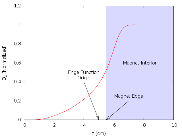
1DProfile1 field map described in Default Field Map (OPAL-t). The exit fringe field of this magnet is the mirror image.So far we have described how to setup an RBEND or SBEND element, but
have not explained how OPAL-t uses this information to calculate the
magnetic field. The field of both types of magnets is divided into three
regions:
-
Entrance fringe field.
-
Central field.
-
Exit fringe field.
This can be seen clearly in Figure 44.
The purpose of the 1DProfile1 field map see 1DProfile1
associated with the element is to define the Enge functions
(Enge function) that model the entrance and exit fringe fields.
To model a particular bend magnet, one must fit the field profile along
the mid-plane of the magnet perpendicular to its face for the entrance
and exit fringe fields to the Enge function:
where \(D\) is the full gap of the magnet, \(N_{order}\) is the Enge function order and \(z\) is the distance from the origin of the Enge function perpendicular to the edge of the dipole. The origin of the Enge function, the order of the Enge function, \(N_{order}\), and the constants \(c_0\) to \(c_{N_{order}}\) are free parameters that are chosen so that the function closely approximates the fringe region of the magnet being modeled. An example of the entrance fringe field is shown in Figure 18.
Let us assume we have a correctly defined positive RBEND or SBEND
element as illustrated in Figure 16 and Figure 17. (As already stated, any
bend can be described by a rotated positive bend.) OPAL-t then has the
following information:
Here, we have defined an overall Enge function, \(F(z)\), with
three parts: entrance, center and exit. The exit and entrance fringe
field regions have the form of Enge function with parameters
defined by the 1DProfile1 field map file given by the element
parameter FMAPFN. Defining the coordinates:
using the conditions
and making the definitions:
we can expand the field off axis, with the result:
These expression are not well suited for numerical calculation, so, we expand them about \(y\) to \(O(y^2)\) to obtain:
-
In fringe field regions:
-
In central region:
These are the expressions OPAL-t uses to calculate the field inside an
RBEND or SBEND. First, a particle’s position inside the bend is
determined (entrance region, center region, or exit region). Depending
on the region, OPAL-t then determines the values of
\(\Delta_x\), \(y\) and \(\Delta_z\), and
then calculates the field values using the above expressions.
11.4.6. Default Field Map (OPAL-t)
Rather than force users to calculate the field of a dipole and then fit
that field to find Enge coefficients for the dipoles in their
simulation, we have a default set of values we use from [24] that are
set when the default field map, 1DPROFILE1-DEFAULT is used:
The same values are used for both the entrance and exit regions of the magnet. In general they will give good results. (Of course, at some point as a beam line design becomes more advanced, one will want to find Enge coefficients that fit the actual magnets that will be used in a given design.)
The default field map is the equivalent of the following custom
1DProfile1 (see 1DProfile1 for an explanation of the field
map format) map:
1DProfile1 5 5 2.0
 -10.0 0.0 10.0 1
 -10.0 0.0 10.0 1
  0.478959
  1.911289
 -1.185953
  1.630554
 -1.082657
  0.318111
  0.478959
  1.911289
 -1.185953
  1.630554
 -1.082657
  0.318111
As one can see, the default magnet gap for 1DPROFILE1-DEFAULT is
set to 2.0 cm. This value can be overridden by the GAP attribute of the
magnet (see RBend (OPAL-t) and SBend (OPAL-t)).
11.4.7. SBend3D (OPAL-cycl)
The SBend3D element enables definition of a bend from 3D field maps.
This can be used in conjunction with the RINGDEFINITION element to
make a ring for tracking through OPAL-cycl.
label: SBEND3D, FMAPFN=string, LENGTH_UNITS=real, FIELD_UNITS=real;
- FMAPFN
-
The field map file name.
- LENGTH_UNITS
-
Units for length (set to 1.0 for units in mm, 10.0 for units in cm, etc).
- FIELD_UNITS
-
Units for field (set to 1.0 for units in T, 0.001 for units in mT, etc).
Field maps are defined using Cartesian coordinates but in a polar geometry. The following conventions have to be fulfilled:
-
3D Field maps have to be generated in the vertical direction (z coordinate in OPAL-cycl) from z = 0 upwards. Maps cannot be generated symmetrically about z = 0 towards negative z values.
-
The field map file must be in the form with columns ordered as follows: [\(x, z, y, B_{x}, B_{z}, B_{y}\)].
-
Grid points of the position and field strength have to be written on a grid in (\(r, z, \theta\)) with the primary direction corresponding to the azimuthal direction, secondary to the vertical direction and tertiary to the radial direction.
SBEND3D assumes a dipole symmetry. In a dipole symmetry, fields below the symmetry plane Z=0 have the same field in the direction perpendicular to the symmetry plane, \(B_{z}\), but field components parallel to the symmetry plane have the opposite direction (sign).
Below are two examples of a SBEND3D which loads a field map file named “90degree_Dipole_Magnet.out” defining a hard edge model of 90 degree dipole magnet with homogenous magnetic field. The first 8 lines are presumed to be header material and are ignored. Positions have units of m and fields units of Tesla. The corresponding 3D magnetic field map is shown in the following figure in the Cartesian coordinate system (x, y, z). A horizontal cross section of the 3D magnetic field map when z = 0 is also shown.
Dipole: SBEND3D, FMAPFN="90degree_Dipole_Magnet.out", LENGTH_UNITS=1000.0, FIELD_UNITS=-10.0;
The first few lines of the field map file are as follows:
	4550000	4550000	4550000	1
X [LENGTH_UNITS]
Z [LENGTH_UNITS]
Y [LENGTH_UNITS]
BX [FIELD_UNITS]
BZ [FIELD_UNITS]
BY [FIELD_UNITS]
0
4.3586435e-01   5.0000000e-02   1.2803431e+00   0.0000000e+00   1.6214000e+00   0.0000000e+00
4.2691532e-01   5.0000000e-02   1.2833548e+00   0.0000000e+00   1.6214000e+00   0.0000000e+00
4.1794548e-01   5.0000000e-02   1.2863039e+00   0.0000000e+00   1.6214000e+00   0.0000000e+00
This is a restricted feature for OPAL-cycl.
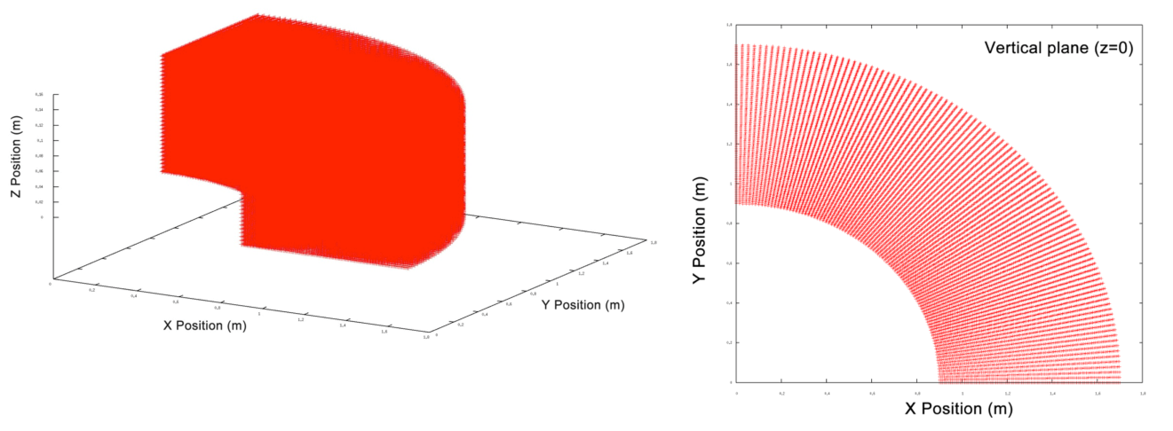
11.5. Quadrupole
label:QUADRUPOLE, TYPE=string, APERTURE=real-vector,
      L=real, K1=real, K1S=real;
The reference system for a quadrupole is a Cartesian coordinate system This is a restricted feature for OPAL-t.
A QUADRUPOLE has the following real attributes:
- K1
-
The normal quadrupole component \(K_1=\frac{\partial B_y}{\partial x}\). The default is 0 \(\mathrm{Tm^{-1}}\). The component is positive, if \(B_y\) is positive on the positive \(x\)-axis. This implies horizontal focusing of positively charged particles which travel in positive \(s\)-direction.
- K1S
-
The skew quadrupole component. \(K_{1s}=-\frac{\partial B_x}{\partial x}\). The default is 0 \(\mathrm{Tm^{-1}}\). The component is negative, if \(B_x\) is positive on the positive \(x\)-axis.
- DK1
-
The normalised quadrupole coefficient error.
- DK1S
-
The normalised skew quadrupole coefficient error.
Example:
QP1: Quadrupole, L=1.20, ELEMEDGE=-0.5265, K1=0.11;
11.6. Sextupole
label: SEXTUPOLE, TYPE=string, APERTURE=real-vector,
       L=real, K2=real, K2S=real;
A SEXTUPOLE has the following real attributes:
- K2
-
The normal sextupole component \(K_2=\frac{\partial{^2} B_y}{\partial x^2}\). The default is 0 \(\mathrm{T m^{-2}}\). The component is positive, if \(B_y\) is positive on the \(x\)-axis.
- K2S
-
The skew sextupole component \(K_{2s}=-\frac{\partial{^2}B_x}{\partial x^{2}}\). The default is 0 \(\mathrm{T m^{-2}}\). The component is negative, if \(B_x\) is positive on the \(x\)-axis.
- DK2
-
The normalised sextupole coefficient error.
- DK2S
-
The normalised skew sextupole coefficient error.
Example:
S:SEXTUPOLE, L=0.4, K2=0.00134;
The reference system for a sextupole is a Cartesian coordinate system
11.7. Octupole
label:OCTUPOLE, TYPE=string, APERTURE=real-vector,
      L=real, K3=real, K3S=real;
An OCTUPOLE has the following real attributes:
- K3
-
The normal octupole component \(K_3=\frac{\partial{^3} B_y}{\partial x^3}\). The default is 0 \(\mathrm{Tm^{-3}}\). The component is positive, if \(B_y\) is positive on the positive \(x\)-axis.
- K3S
-
The skew octupole component \(K_{3s}=-\frac{\partial{^3}B_x}{\partial x^{3}}\). The default is 0 \(\mathrm{Tm^{-3}}\). The component is negative, if \(B_x\) is positive on the positive \(x\)-axis.
- DK3
-
The normalised octupole coefficient error.
- DK3S
-
The normalised skew octupole coefficient error.
Example:
O3:OCTUPOLE, L=0.3, K3=0.543;
The reference system for an octupole is a Cartesian coordinate system
11.8. General Multipole
The MULTIPOLE element defines a thick multipole.
If the length is non-zero, the strengths are per unit
length. If the length is zero, the strengths are the
values integrated over the length.
With zero length no synchrotron radiation can be calculated.
A MULTIPOLE in OPAL-t is of arbitrary order.
label:MULTIPOLE, TYPE=string, APERTURE=real-vector,
      L=real, KN=real-vector, KS=real-vector;
- KN
-
A real vector see Arrays, containing the normal multipole coefficients, \(K_n=\frac{\partial{^n} B_y}{\partial x^n}\). (default is 0 \(\mathrm{Tm^{-n}}\)). A component is positive, if \(B_y\) is positive on the positive \(x\)-axis.
- KS
-
A real vector see Arrays, containing the skew multipole coefficients, \(K_{n~s}=-\frac{\partial{^n}B_x}{\partial x^{n}}\). (default is 0 \(\mathrm{Tm^{-n}}\)). A component is negative, if \(B_x\) is positive on the positive \(x\)-axis.
- DKN
-
A real vector see Arrays, containing the normal normalised multipole strength errors. (default is 0 \(\mathrm{Tm^{-n}}\)).
- DKS
-
A real vector see Arrays, containing the skew normalised multipole strength errors. (default is 0 \(\mathrm{Tm^{-n}}\)).
The number of poles of each component is (\(2 n + 2\)).
Superposition of many multipole components is permitted. The reference system for a multipole is a Cartesian coordinate system
The following example is equivalent to the quadruple example in Quadrupole.
M27:MULTIPOLE, L=1, ELEMEDGE=3.8, KN={0.0,0.11};
A multipole has no effect on the reference orbit, i.e. the reference system at its exit is the same as at its entrance. Use the dipole component only to model a defective multipole.
11.9. General Multipole (will replace General Multipole when implemented)
A MULTIPOLET is in OPAL-cycl a general multipole with extended
features. It can represent a straight or curved magnet. In the curved
case, the user may choose between constant or variable radius. This
model includes fringe fields. The detailed description can be found at:
https://gitlab.psi.ch/OPAL/src/uploads/0d3fc561b57e8962ed79a57cd6115e37/8FBB32A4-7FA1-4084-A4A7-CDDB1F949CD3_psi.ch.pdf.
Label:MULTIPOLET, L=real, ANGLE=real, VAPERT=real, HAPERT=real,
      LFRINGE=real, RFRINGE=real, TP=real-vector, VARRADIUS=bool;
- L
-
Physical length of the magnet (meters), without end fields. (Default: 1 m)
- ANGLE
-
Physical angle of the magnet (radians). If not specified, the magnet is considered to be straight (ANGLE=0.0). This is not the total bending angle since the end fields cause additional bending. The radius of the multipole is set from the LENGTH and ANGLE attributes.
- VAPERT
-
Vertical (non-bend plane) aperture of the magnet (meters). (Default: 0.5 m)
- HAPERT
-
Horizontal (bend plane) aperture of the magnet (meters). (Default: 0.5 m)
- LFRINGE
-
Length of the left fringe field (meters). (Default: 0.0 m)
- RFRINGE
-
Length of the right fringe field (meters). (Default: 0.0 m)
- TP
-
A real vector see Arrays, containing the multipole coefficients of the field expansion on the mid-plane in the body of the magnet: the transverse profile \( T(x) = B_0 + B_1 x + B_2 x^2 + \ldots \) is set by TP=\(B_0\), \(B_1\), \(B_2\) (units: \( T \cdot m^{-n}\)). The order of highest multipole component is arbitrary, but all components up to the maximum must be given, even if they are zero.
- MAXFORDER
-
The order of the maximum function \(f_n\) used in the field expansion (default: 5). See the scalar magnetic potential below. This sets for example the maximum power of \(z\) in the field expansion of vertical component \(B_z\) to \(2 \cdot \text{MAXFORDER} \).
- EANGLE
-
Entrance edge angle (radians).
- ROTATION
-
Rotation of the magnet about its central axis (radians, counterclockwise). This enables to obtain skew fields. (Default 0.0 rad)
- VARRADIUS
-
This is to be set TRUE if the magnet has variable radius. More precisely, at each point along the magnet, its radius is computed such that the reference trajectory always remains in the centre of the magnet. In the body of the magnet the radius is set from the LENGTH and ANGLE attributes. It is then continuously changed to be proportional to the dipole field on the reference trajectory while entering the end fields. This attribute is only to be set TRUE for a non-zero dipole component. (Default: FALSE)
- VARSTEP
-
The step size (meters) used in calculating the reference trajectory for VARRARDIUS = TRUE. It specifies how often the radius of curvature is re-calculated. This has a considerable effect on tracking time. (Default: 0.1 m)
Superposition of many multipole components is permitted. The reference system for a multipole is a Cartesian coordinate system for straight geometry and a \((x,s,z)\) Frenet-Serret coordinate system for curved geometry. In the latter case, the axis \(\hat{s}\) is the central axis of the magnet.
The following example shows a combined function magnet with a dipole component of 2 Tesla and a quadrupole gradient of 0.1 Tesla/m.
M30:MULTIPOLET, L=1, RFRINGE=0.3, LFRINGE=0.2, ANGLE=PI/6, TP={2.0, 0.1}, VARRADIUS=TRUE;
The field expansion used in this model is based on the following scalar potential:
Mid-plane symmetry is assumed and the vertical component of the field on the mid-plane is given by the user under the form of the transverse profile \(T(x)\). The full expression for the vertical component is then
where \(S(s)\) is the fringe field. This element uses the Tanh model for the end fields, having only three parameters (the centre length \(s_0\) and the fringe field lengths \(\lambda_{left}\), \(\lambda_{right}\)):
Starting from Maxwell’s laws, the functions \(f_n\) are computed recursively and finally each component of the magnetic field is obtained from \(V\) using the corresponding geometries.
11.10. Solenoid
label:SOLENOID, TYPE=string, APERTURE=real-vector,
      L=real, KS=real;
A SOLENOID has two real attributes:
- KS
-
The solenoid strength \(K_s=\frac{\partial B_s}{\partial s}\), default is 0 \(\mathrm{Tm^{-1}}\). For positive
KSand positive particle charge, the solenoid field points in the direction of increasing \(s\).
The reference system for a solenoid is a Cartesian coordinate system Using a solenoid in OPAL-t mode, the following additional parameters are defined:
- FMAPFN
-
Field maps must be specified.
Example:
SP1: Solenoid, L=1.20, ELEMEDGE=-0.5265, KS=0.11,
     FMAPFN="1T1.T7";
11.11. Cyclotron
label:CYCLOTRON, TYPE=string, CYHARMON=int,
      PHIINIT=real, PRINIT=real, RINIT=real,
      SYMMETRY=real, RFFREQ=real, FMAPFN=string;
A CYCLOTRON object includes the main characteristics of a cyclotron,
the magnetic field, and also the initial condition of the injected
reference particle, and it has currently the following attributes:
- TYPE
-
The data format of field map. Currently the following formats are implemented: RING (PSI format), CARBONCYCL, CYCIAE, AVFEQ, FFA and BANDRF. For the details of their data format, please read Field Maps.
- CYHARMON
-
The harmonic number of the cyclotron \(h\).
- RFFREQ
-
The RF system \(f_{rf}\) (unit:MHz, default: 0). The particle revolution frequency \(f_{rev}\) = \(f_{rf}\) / \(h\).
- FMAPFN
-
File name for the magnetic field map. BSCALE: Scale factor for the magnetic field map.
- SYMMETRY
-
Defines symmetrical fold number of the B field map data.
- GEOMETRY
-
Defines the boundary geometry in order to use it for particle termination (see Chapter Geometry). The particles hitting on the
GEOMETRYwill be deleted, and they are recorded in the HDF5 file <GEOM>.h5 (or ASCII ifASCIIDUMPis true). - FMLOWE
-
Minimal energy [GeV] the fieldmap can accept. Used in
GAUSSMATCHEDdistribution. - FMHIGHE
-
Maximal energy [GeV] the fieldmap can accept. Used in
GAUSSMATCHEDdistribution. - RINIT
-
The initial radius of the reference particle (unit: mm, default: 0)
- PHIINIT
-
The initial azimuth of the reference particle (unit: degree, default: 0)
- ZINIT
-
The initial axial position of the reference particle (unit: mm, default: 0)
- PRINIT
-
Initial radial momentum of the reference particle \(P_r=\beta_r\gamma\) (default : 0)
- PZINIT
-
Initial axial momentum of the reference particle \(P_z=\beta_z\gamma\) (default : 0)
- MINZ
-
The minimal vertical extent of the machine (unit: mm, default : -10000.0)
- MAXZ
-
The maximal vertical extent of the machine (unit: mm, default : 10000.0)
- MINR
-
Minimal radial extent of the machine (unit: mm, default : 0.0)
- MAXR
-
Minimal radial extent of the machine (unit: mm, default : 10000.0)
During the tracking, the particle (\(r, z, \theta\)) will be
deleted if MINZ \(< z <\) MAXZ or MINR \(< r <\)
MAXR, and it will be recorded in the HDF5 file OUTFN.h5
(or ASCII if ASCIIDUMP is true),
(see Common Attributes).
Example:
ring: Cyclotron, TYPE="RING", CYHARMON=6, PHIINIT=0.0,
      PRINIT=-0.000240, RINIT=2131.4, SYMMETRY=8.0,
      RFFREQ=50.650, FMAPFN="s03av.nar",
      MAXZ=10, MINZ=-10, MINR=0, MAXR=2500;
If TYPE is set to BANDRF, the 3D electric field map of RF cavity will be
read from external H5Hut file and the following extra
arguments need to specified:
- RFMAPFN
-
The file name(s) for the electric field map(s) in H5Hut binary format.
- RFPHI
-
The initial phase(s) of the electric field map(s) (rad)
- RFFREQ
-
The frequencies of the electric field maps. 0 indicates a constant field.
- ESCALE
-
The scale factor(s) for the electric field map(s)
- SUPERPOSE
-
An option whether the electric field map(s) is superposed (see also below).
Example for single electric field map:
COMET: Cyclotron, TYPE="BANDRF", CYHARMON=2, PHIINIT=-71.0,
PRINIT=pr0, RINIT=r0, SYMMETRY=1.0, FMAPFN="Tosca_map.txt",
RFPHI=Pi, RFFREQ=72.0,  RFMAPFN="efield.h5part",
ESCALE=1.06E-6;
We can have more than one RF field maps.
Example for multiple RF field maps:
COMET: Cyclotron, TYPE="BANDRF", CYHARMON=2, PHIINIT=-71.0,
PRINIT=pr0, RINIT=r0, SYMMETRY=1.0, FMAPFN="Tosca_map.txt",
RFPHI={Pi,0,Pi,0}, RFFREQ={72.0,72.0,72.0,72.0},
RFMAPFN={"e1.h5part","e2.h5part","e3.h5part","e4.h5part"},
ESCALE={1.06E-6, 3.96E-6,1.3E-6,1.E-6}, SUPERPOSE={true,false,false,true};
If SUPERPOSE is set to true and if a particle is located in the field region, the field is always applied. If SUPERPOSE is set to false, then only one field map with SUPERPOSE false is applied, the one which has highest priority, is used to do interpolation for the particle tracking. The priority ranking is decided by their sequence in the list of RFMAPFN argument, i.e., "e1.h5part" has the highest priority and "e4.h5part" has the lowest priority.
Another method to model an RF cavity is to read the RF voltage profile in the RFCAVITY element see RF Cavities (OPAL-t and OPAL-cycl) and make a momentum kick when a particle crosses the RF gap. In the center region of the compact cyclotron, the electric field shape is complicated and may make a significant impact on transverse beam dynamics. Hence a simple momentum kick is not enough and we need to read 3D field map to do precise simulation.
In addition, a trim-coil field model is also implemented to do fine tuning on the magnetic field. The trimcoils can be added with:
- TRIMCOIL
-
Array of the trim coil names
A TRIMCOIL object can be defined in two ways:
- TYPE
-
Type specifies PSI-BFIELD, PSI-PHASE or PSI-BFIELD-MIRRORED trim coil descriptions. The general PSI-BFIELD and PSI-PHASE descriptions are based on rational functions with polynomials in the nominator and the denominator. The function describes the magnetic field [T] resp. the phase shift as function of the radius [mm]. Separate functions can be given for the radial and azimuthal direction. These functions are multiplied together for the function. If a function in a direction is not specified it is the identity 1. The PSI-BFIELD-MIRRORED type is described in http://accelconf.web.cern.ch/AccelConf/ipac2017/papers/thpab077.pdf.
- RMIN
-
Inner radius of the trim coil [mm]
- RMAX
-
Outer radius of the trim coil [mm]
- PHIMIN
-
Minimal azimuth [deg] (default 0) (not for PSI-BFIELD-MIRRORED)
- PHIMAX
-
Maximal azimuth [deg] (default 360) (not for PSI-BFIELD-MIRRORED)
- BMAX
-
Maximal B field of the trim coils [T] (for PSI-BFIELD) or maximal phase shift (for PSI-PHASE)
- COEFNUM
-
Coefficients of the numerator for the radial direction, first coefficient is zeroth order. If COEFNUMPHI is not specified, the numerator is 1 (not for PSI-BFIELD-MIRRORED).
- COEFDENOM
-
Coefficients of the denominator for the radial direction, first coefficient is zeroth order. If COEFDENOM is not specified, the denominator is 1, and the description will be a normal polynom (not for PSI-BFIELD-MIRRORED).
- COEFNUMPHI
-
Coefficients of the numerator for the azimuthal direction, first coefficient is zeroth order. If COEFNUMPHI is not specified, the numerator is 1. (not for PSI-BFIELD-MIRRORED).
- COEFDENOMPHI
-
Coefficients of the denominator for the azimuthal direction, first coefficient is zeroth order. If COEFDENOMPHI is not specified, the denominator is 1, and the description will be a normal polynom (not for PSI-BFIELD-MIRRORED).
- SLPTC
-
Slopes of the rising edge [1/mm] (for PSI-BFIELD-MIRRORED type only)
Example:
tc1:  TRIMCOIL, TYPE="PSI-BFIELD-MIRRORED", RMIN = 2022.09, RMAX = 2132.09, BMAX=2.0e-4, SLPTC=1;
tc15: TRIMCOIL, TYPE="PSI-BFIELD",          RMIN = 3000,    RMAX = 4500,    BMAX=13e-4,
      COEFNUM   = {-0.426038643356, 0.311242287271, -0.0484487029431},
      COEFDENOM = {19.3541404562, -22.2057165548, 9.99489842329, -2.00909633025, 0.14942099903};

Ring: CYCLOTRON, TYPE="RINGCYC", CYHARMON=6, PHIINIT=0.0, PRINIT=0.0,
      RINIT=2131, SYMMETRY=8.0, RFFREQ=50.65, BSCALE=1, FMAPFN="s03av.nar",
      TRIMCOIL={tc1, tc15};
This is a restricted feature: OPAL-cycl.
11.12. FFA Magnet
OPAL supports two analytical field models that describe FFA magnets. SCALINGFFAMAGNET generates a sector FFA magnet that scales radially. VERTICALFFAMAGNET generates a vertical FFA magnet that scales vertically.
11.12.1. Scaling FFA Magnet
The scaling FFA magnet is a fully scaling field model that includes scaling fringe fields. A scaling FFA magnet has a field profile like
where \(r\) and \(z\) are cylindrical polar coordinates, \(\psi = \phi - \tan(\delta) \ln(r/r_0)\) is the azimuthal angle in the spiral coordinate system, \(delta\), \(r_0\) and \(k\) are geometrical constants that define the magnet field dependence and \(B_0\) is the dipole field strength of the magnet at radius \(r_0\). In OPAL, \(f_0\) is a \(tanh\) function and higher order terms are chosen so as to satisfy Maxwell’s equations.
- B0
-
The nominal dipole field of the magnet [T].
- R0
-
Radial scale [m].
- FIELD_INDEX
-
The scaling magnet field index.
- TAN_DELTA
-
Tangent of the spiral angle; set to 0 to make a radial sector magnet.
- MAX_Y_POWER
-
The maximum power in y that will be considered in the field expansion.
- END_LENGTH
-
The end length of the spiral FFA [m].
- HEIGHT
-
Full height of the magnet. Particles moving more than height/2. off the midplane (either above or below) are out of the aperture [m].
- CENTRE_LENGTH
-
The centre length of the spiral FFA [m].
- RADIAL_NEG_EXTENT
-
Particles are considered outside the tracking region if radius is less than R0-RADIAL_NEG_EXTENT [m].
- RADIAL_POS_EXTENT
-
Particles are considered outside the tracking region if radius is greater than R0+RADIAL_POS_EXTENT [m].
- MAGNET_START
-
Determines the position of the central portion of the magnet field relative to the element start (default is 2*end_length). [m].
- MAGNET_END
-
Offset to the end of the magnet, i.e. placement of the next element. Default is centre_length + 4*end_length.
- AZIMUTHAL_EXTENT
-
The field will be assumed zero if particles are more than AZIMUTHAL_EXTENT from the magnet centre (psi=0). Default is CENTRE_LENGTH/2.+5.*END_LENGTH [m].
This is a restricted feature: OPAL-cycl.
11.12.2. Vertical FFA Magnet
The VERTICALFFAMAGNET is a fully scaling field model that includes scaling fringe fields. A vertical FFA magnet has a field profile like
where \(m\) and \(B_0\) are magnet parameters, \(f_0\) is a \(tanh\) function and higher order terms are chosen so as to satisfy Maxwell’s equations. The field parameters can be specified in the OPAL input file using the following parameters
- B0
-
The nominal dipole field of the magnet at z = 0, \(B_0\) [T].
- FIELD_INDEX
-
The scaling magnet field index, \(m\) [m^-1].
- MAX_Y_POWER
-
The maximum power in y that will be considered in the field expansion.
- END_LENGTH
-
The end length of the VFFA [m].
- CENTRE_LENGTH
-
The centre length of the VFFA [m].
- WIDTH
-
The full width of the magnet. Particles moving more than WIDTH/2 horizontally, in either direction, are considered out of the tracking region [m].
- HEIGHT_NEG_EXTENT
-
Particles are considered outside the tracking region if height is less than HEIGHT_NEG_EXTENT [m].
- HEIGHT_POS_EXTENT
-
Particles are considered outside the tracking region if height is greater than HEIGHT_POS_EXTENT [m].
- BB_LENGTH
-
The total length of the bounding box. The magnet will be placed symmetrically in the bounding box [m].
VERTICALFFAMAGNET is rectangular; the next element will be placed BB_LENGTH from the start position of the VERTICALFFAMAGNET.
This is a restricted feature: OPAL-cycl.
11.13. Ring Definition
label: RINGDEFINITION,
       RFFREQ=real, HARMONIC_NUMBER=real, IS_CLOSED=string, SYMMETRY=int,
       LAT_RINIT=real, LAT_PHIINIT=real, LAT_THETAINIT=real,
       BEAM_PHIINIT=real, BEAM_PRINIT=real, BEAM_RINIT=real;
A RingDefinition object contains the main characteristics of a
generalized ring. The RingDefinition lists characteristics of the
entire ring such as harmonic number together with the position of the
initial element and the position of the reference trajectory.
The RingDefinition can be used in combination with SBEND3D, offsets
and VARIABLE_RF_CAVITY elements to make up a complete ring.
- RFFREQ
-
Nominal RF frequency of the ring [MHz].
- HARMONIC_NUMBER
-
The harmonic number of the ring - i.e. number of bunches in a single pass.
- SYMMETRY
-
Azimuthal symmetry of the ring. Ring elements will be placed repeatedly
SYMMETRYtimes. - IS_CLOSED
-
Set to
FALSEto disable checking for ring closure. - LAT_RINIT
-
Radius of the first element placement in the lattice [m].
- LAT_PHIINIT
-
Azimuthal angle of the first element placed in the lattice [degree].
- LAT_THETAINIT
-
Angle in the mid-plane relative to the ring tangent for placement of the first element [degree].
- BEAM_RINIT
-
Initial radius of the reference trajectory [m].
- BEAM_PHIINIT
-
Initial azimuthal angle of the reference trajectory [degree].
- BEAM_PRINIT
-
Transverse momentum \(\beta \gamma\) for the reference trajectory.
In the following example, we define a ring with radius 2.35 m and 4 cells.
ringdef: RINGDEFINITION, HARMONIC_NUMBER=6, LAT_RINIT=2350.0, LAT_PHIINIT=0.0,
         LAT_THETAINIT=0.0, BEAM_PHIINIT=0.0, BEAM_PRINIT=0.0,
         BEAM_RINIT=2266.0, SYMMETRY=4.0, RFFREQ=0.2;
11.13.1. Local Cartesian Offset
The LOCAL_CARTESIAN_OFFSET enables the user to place an object at an
arbitrary position in the coordinate system of the preceding element.
This enables drift spaces and placement of overlapping elements.
- END_POSITION_X
-
x position of the next element start in the coordinate system of the preceding element [m].
- END_POSITION_Y
-
y position of the next element start in the coordinate system of the preceding element [m].
- END_NORMAL_X
-
x component of the normal vector defining the placement of the next element in the coordinate system of the preceding element [m].
- END_NORMAL_Y
-
y component of the normal vector defining the placement of the next element in the coordinate system of the preceding element [m].
11.13.2. Local Cylindrical Offset
The LOCAL_CYLINDRICAL_OFFSET enables the user to place an object at an
arbitrary position in the coordinate system of the preceding element in cylindrical coordinates.
This enables drift spaces and placement of overlapping elements.
- THETA_IN
-
Angle between the previous element and the displacement vector [rad].
- THETA_OUT
-
Angle between the displacement vector and the next element [rad].
- LENGTH
-
Length of the offset [m].
11.14. Source (OPAL-t)
Its first purpose is to indicate that the particles are emitted from a gun.
This is needed to place the elements in three-dimensional space. Its second
purpose is to delete impacting particles that are propagating in reverse
direction. This function is optional and can be controlled with the parameter
TRANSPARENT. The particles hitting on the source are recorded in the OUTFN
file (see Common Attributes). The SOURCE
element only works in OPAL-t.
- TRANSPARENT
-
Boolean to indicate whether impacting particles can propagate further. Its default is
FALSEsuch that the particles are deleted.
11.15. RF Cavities (OPAL-t and OPAL-cycl)
For an RFCAVITY the three modes have four real attributes in common:
label:RFCAVITY, APERTURE=real-vector, L=real,
      VOLT=real, LAG=real;
- L
-
The length of the cavity (default: 0 m)
- VOLT
-
The peak RF voltage (default: 0 MV). The effect of the cavity is \(\delta E=\mathrm{VOLT}\cdot\sin(2\pi(\mathrm{LAG}-\mathrm{HARMON}\cdot f_0 t))\).
- LAG
-
The phase lag [rad] (default: 0). In OPAL-t this phase is in general relative to the phase at which the reference particle gains the most energy. This phase is determined using an auto-phasing algorithm (see Appendix Auto-phasing Algorithm). This auto-phasing algorithm can be switched off, see
APVETO. - DLAG
-
The phase lag error [rad] (default: 0).
11.15.1. OPAL-t mode
Using a RF Cavity in OPAL-t mode, the following additional parameters are defined:
- FMAPFN
-
Field maps in the T7 format can be specified.
- TYPE
-
Type specifies
STANDING[default] orSINGLEGAPstructures. - FREQ
-
Defines the frequency of the RF Cavity in units of MHz. A warning is issued when the frequency of the cavity card does not correspond to the frequency defined in the FMAPFN file. The frequency of the cavity card overrides the frequency defined in the FMAPFN file.
- APVETO
-
If
TRUEthis cavity will not be auto-phased. Instead the phase of the cavity is equal toLAGat the arrival time of the reference particle (arrival at the limit of its field not atELEMEDGE).
Example standing wave cavity which mimics a DC gun:
gun: RFCavity, L=0.018, VOLT=-131/(1.052*2.658),
     FMAPFN="1T3.T7", ELEMEDGE=0.00,
     TYPE="STANDING", FREQ=1.0e-6;
Example of a two frequency standing wave cavity:
rf1: RFCavity, L=0.54, VOLT=19.961, LAG=193.0/360.0,
     FMAPFN="1T3.T7", ELEMEDGE=0.129, TYPE="STANDING",
     FREQ=1498.956;
rf2: RFCavity, L=0.54, VOLT=6.250, LAG=136.0/360.0,
     FMAPFN="1T4.T7", ELEMEDGE=0.129, TYPE="STANDING",
     FREQ=4497.536;
11.15.2. OPAL-cycl mode
Using a RF Cavity (standing wave) in OPAL-cycl mode, the following parameters are defined:
- FMAPFN
-
Name of file which stores normalized voltage amplitude curve of cavity gap in ASCII format. (See data format in RF field)
- VOLT
-
Peak value of voltage amplitude curve in MV.
- TYPE
-
Defines Cavity type,
SINGLEGAPrepresents cyclotron type cavity. - FREQ
-
Frequency of the RF Cavity in units of MHz.
- RMIN
-
Radius of the cavity inner edge in mm.
- RMAX
-
Radius of the cavity outer edge in mm.
- ANGLE
-
Azimuthal position of the cavity in global frame in degree.
- PDIS
-
Perpendicular distance (impact parameter) of cavity from center of cyclotron in mm. If its value is positive, the radius increases clockwise (larger radius has smaller azimuthal angle).
- GAPWIDTH
-
Set gap width of cavity in mm.
- PHI0
-
Set initial phase of cavity in degree.
Example of a RF cavity of cyclotron:
rf0: RFCavity, VOLT=0.25796, FMAPFN="Cav1.dat",
     TYPE="SINGLEGAP", FREQ=50.637, RMIN = 350.0,
     RMAX = 3350.0, ANGLE=35.0,   PDIS = 0.0,
     GAPWIDTH = 0.0, PHI0=phi01;
Figure 20 shows the simplified geometry of a cavity gap and its parameters.
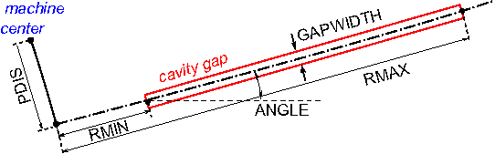
11.16. RF Cavities with Time Dependent Parameters
The VARIABLE_RF_CAVITY element can be used to define RF Cavities with
Time Dependent Parameters in OPAL-cycl mode. Variable RF Cavities must
be placed using the RingDefinition element.
- FREQUENCY_MODEL
-
String naming the time dependence model of the cavity frequency, \(f\) [MHz].
- AMPLITUDE_MODEL
-
String naming the time dependence model of the cavity amplitude, \(E_0\) [MV/m].
- PHASE_MODEL
-
String naming the time dependence model of the cavity phase offset, \(\phi\) [rad].
- WIDTH
-
Full width of the cavity [m].
- HEIGHT
-
Full height of the cavity [m].
- L
-
Full length of the cavity [m].
The field inside the cavity is given by
with no field outside the cavity boundary. There is no magnetic field or transverse dependence on electric field.
11.16.1. Time Dependence
Polynomial Time Dependence
The POLYNOMIAL_TIME_DEPENDENCE element is used to define time
dependent parameters in RF cavities in terms of a third order
polynomial.
- P0
-
Constant term in the polynomial expansion.
- P1
-
First order term in the polynomial expansion [ns\(^{-1}\)].
- P2
-
Second order term in the polynomial expansion [ns\(^{-2}\)].
- P3
-
Third order term in the polynomial expansion [ns\(^{-3}\)].
The polynomial is evaluated as
An example of a Variable Frequency RF cavity of cyclotron with polynomial time dependence of parameters is given below:
Spline Time Dependence
The SPLINE_TIME_DEPENDENCE element is used to define time
dependent parameters in RF cavities in terms of a first or third order
spline fit.
- ORDER
-
Order of the lookup - either 1 for linear interpolation, or 3 for cubic interpolation with quadratic smoothing. Other values make an error.
- TIMES
-
Array of real times in ns. There must be at least
ORDER+1 elements in the array and they must be strictly monotonically increasing. - VALUES
-
Array of real values. The length of
VALUESmust be the same as the length ofTIMES.
11.16.2. Fringe Field
It is possible to model a soft-edged RF cavity with time dependent parameters using the VARIABLE_RF_CAVITY_FRINGE_FIELD element. This will place a full cavity including the field body and fringe fields. VARIABLE_RF_CAVITY_FRINGE_FIELD must be placed using the RingDefinition element.
- FREQUENCY_MODEL
-
String naming the time dependence model of the cavity frequency, \(f\) [MHz].
- AMPLITUDE_MODEL
-
String naming the time dependence model of the cavity amplitude, \(E_0\) [MV/m].
- PHASE_MODEL
-
String naming the time dependence model of the cavity phase offset, \(\phi\) [rad].
- WIDTH
-
Full width of the cavity [m].
- HEIGHT
-
Full height of the cavity [m].
- L
-
Full length of the cavity bounding box [m].
- CENTRE_LENGTH
-
Length of the cavity field flat top [m].
- END_LENGTH
-
E-fold Length of the cavity field ends [m].
- CAVITY_CENTRE
-
Position of the centre of the cavity relative to the start [m].
- MAX_ORDER
-
Maximum power in vertical coordinate z to which the field will be evaluated.
REAL phi=2.*PI*0.25;

REAL rf_p0=0.00158279;
REAL rf_p1=9.02542e-10;
REAL rf_p2=-1.96663e-16;
REAL rf_p3=2.45909e-23;

RF_FREQUENCY: POLYNOMIAL_TIME_DEPENDENCE, P0=rf_p0, P1=rf_p1,   P2=rf_p2, P3=rf_p3;
RF_AMPLITUDE: POLYNOMIAL_TIME_DEPENDENCE, P0=1.0;
RF_PHASE: POLYNOMIAL_TIME_DEPENDENCE, P0=phi;

HARD_RF_CAVITY: VARIABLE_RF_CAVITY,
           PHASE_MODEL="RF_PHASE", AMPLITUDE_MODEL="RF_AMPLITUDE",
           FREQUENCY_MODEL="RF_FREQUENCY", L=0.100, HEIGHT=0.200, WIDTH=2.000;

SOFT_RF_CAVITY: VARIABLE_RF_CAVITY_FRINGE_FIELD,
           PHASE_MODEL="RF_PHASE", AMPLITUDE_MODEL="RF_AMPLITUDE",
           FREQUENCY_MODEL="RF_FREQUENCY", L=0.200, HEIGHT=0.200, WIDTH=2.000
           CENTRE_LENGTH=0.1, END_LENGTH=0.01, CAVITY_CENTRE=0.1, MAX_ORDER=4;
11.17. Traveling Wave Structure
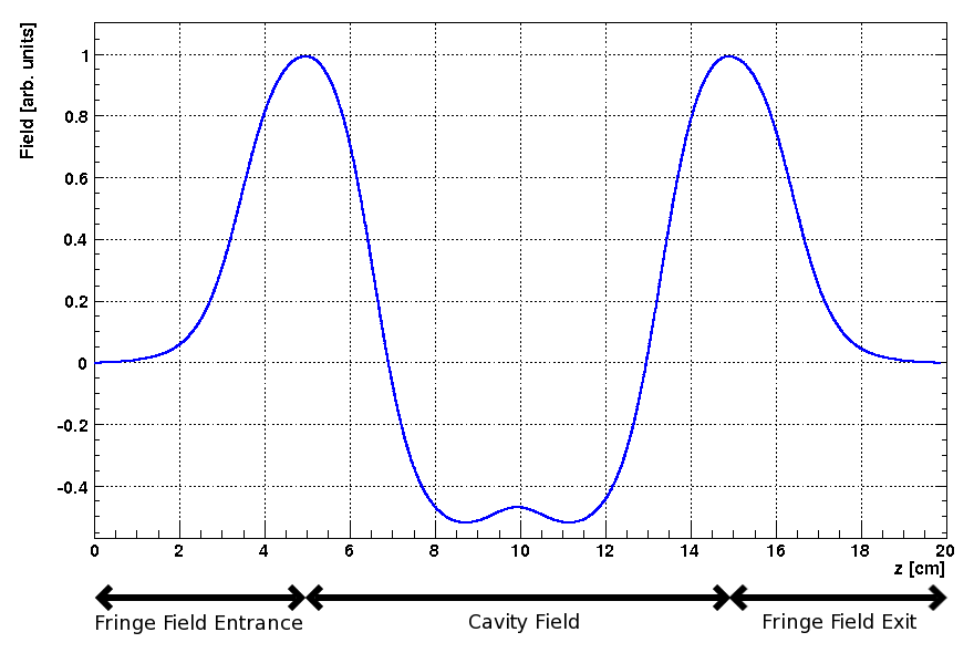
TRAVELINGWAVE structure. The field of a single cavity is shown between its entrance and exit fringe fields. The fringe fields extend one half wavelength (\(\lambda/2\)) to either side.An example of a 1D TRAVELINGWAVE structure field map is shown in
Figure 21. This map is a standing wave solution generated
by Superfish and shows the field on axis for a single accelerating
cavity with the fringe fields of the structure extending to either side.
OPAL-t reads in this field map and constructs the total field of the
TRAVELINGWAVE structure in three parts: the entrance fringe field, the
structure fields and the exit fringe field.
The fringe fields are treated as standing wave structures and are given by:
where VOLT and FREQ are the field magnitude and frequency attributes (see below). \( \phi_{entrance}= \mathrm{LAG}\), the phase attribute of the element (see below). \( \phi_{exit} \) is dependent upon both LAG and the NUMCELLS attribute (see below) and is calculated internally by OPAL-t.
The field of the main accelerating structure is reconstructed from the center section of the standing wave solution shown in Figure 21 using
where d is the cell length and is defined as \(\text{d} = \lambda \cdot \mathrm{MODE} \). MODE is an attribute of the element (see below). When calculating the field from the map (\(\mathbf{E_{from-map}}(x,y,z)\)), the longitudinal position is referenced to the start of the cavity fields at \(\frac{\lambda}{2}\) (In this case starting at \(z = {5.0}cm\)). If the longitudinal position advances past the end of the cavity map (\(\frac{3\lambda}{2} = {15.0}cm\) in this example), an integer number of cavity wavelengths is subtracted from the position until it is back within the map’s longitudinal range.
A TRAVELINGWAVE structure has seven real attributes, one integer
attribute, one string attribute and one Boolean attribute:
label:TRAVELINGWAVE, APERTURE=real-vector, L=real,
      VOLT=real, LAG=real, FMAPFN=string,
      ELEMEDGE=real, FREQ=real, NUMCELLS=integer,
      MODE=real;
- L
-
The length of the cavity (default: 0 m). In OPAL-t this attribute is ignored, the length is defined by the field map and the number of cells.
- VOLT
-
The peak RF voltage (default: 0 MV). The effect of the cavity is \(\delta E=\mathrm{VOLT}\cdot\sin(\mathrm{LAG}- 2\pi\cdot\mathrm{FREQ}\cdot t)\).
- LAG
-
The phase lag [rad] (default: 0). In OPAL-t this phase is in general relative to the phase at which the reference particle gains the most energy. This phase is determined using an auto-phasing algorithm (see Appendix Auto-phasing Algorithm). This auto-phasing algorithm can be switched off, see
APVETO. - DLAG
-
The phase lag error [rad] (default: 0).
- FMAPFN
-
Field maps in the T7 format can be specified.
- FREQ
-
Defines the frequency of the traveling wave structure in units of MHz. A warning is issued when the frequency of the cavity card does not correspond to the frequency defined in the FMAPFN file. The frequency defined in the FMAPFN file overrides the frequency defined on the cavity card.
- NUMCELLS
-
Defines the number of cells in the tank. (The cell count should not include the entry and exit half cell fringe fields.)
- MODE
-
Defines the mode in units of \(2\pi\), for example \(\frac{1}{3}\) stands for a \(\frac{2 \pi}{3}\) structure.
- FAST
-
If FAST is true and the provided field map is in 1D then a 2D field map is constructed from the 1D on-axis field, see Fieldmaps Types and Format. To track the particles the field values are interpolated from this map instead of using an FFT based algorithm for each particle and each step. (default: FALSE)
- APVETO
-
If
TRUEthis cavity will not be auto-phased. Instead the phase of the cavity is equal toLAGat the arrival time of the reference particle (arrival at the limit of its field not atELEMEDGE).
Use of a traveling wave requires the particle momentum P and the
particle charge CHARGE to be set on the relevant optics command before
any calculations are performed.
Example of a L-Band traveling wave structure:
lrf0: TravelingWave, L=0.0253, VOLT=14.750,
      NUMCELLS=40, ELEMEDGE=2.73066,
      FMAPFN="INLB-02-RAC.Ez", MODE=1/3,
      FREQ=1498.956, LAG=248.0/360.0;
11.18. Monitor
A MONITOR detects all particles passing it and writes the position,
the momentum and the time when they hit it into an H5hut file.
Furthermore the exact position of the monitor is stored. It has always a
length of 1 cm consisting of 0.5 cm drift, the monitor of zero length and
another 0.5 cm drift. This is to prevent OPAL-t from missing any
particle. The positions of the particles on the monitor are interpolated
from the current position and momentum one step before they would passe
the monitor.
The attribute OUTFN defines the file into which the monitor should write
the collected data (see Common Attributes).
The file is an H5hut file.
If the attribute TYPE is set to TEMPORAL then the data of all
particles are written to the H5hut file when the reference particle hits
the monitor.
This is a restricted feature for OPAL-t.
11.19. Collimators
Four types of collimators are defined:
- ECOLLIMATOR
-
Elliptic aperture,
- RCOLLIMATOR
-
Rectangular aperture.
- FLEXIBLECOLLIMATOR
-
Description of shape and location of holes can be provided
- CCOLLIMATOR
-
Radial rectangular collimator in cyclotrons
label:ECOLLIMATOR, TYPE=string, APERTURE=real-vector,
      L=real, XSIZE=real, YSIZE=real;

label:RCOLLIMATOR,TYPE=string, APERTURE=real-vector,
      L=real, XSIZE=real, YSIZE=real;

label:FLEXIBLECOLLIMATOR, APERTURE=real-vector,
      L=real, DESCRIPTION=string, FNAME=string, OUTFN=string;
Each type has the following general attributes (available for both OPAL-t and OPAL-cycl collimators):
- OUTFN
-
The file name into which the collimator should write the collected data. If this attribute is empty, the file will be named as the element label. The file is an H5hut file (or ASCII if
ASCIIDUMPis true). - PARTICLEMATTERINTERACTION
-
PARTICLEMATTERINTERACTIONis an attribute of the element (see Chapter Particle Matter Interaction).TYPE=SCATTERINGmust be selected to include scattering interactions and energy loss calculation through theMATERIALdefinition (see Available Materials in OPAL). If this is not set, the particle-matter interaction module will not be activated. Then, the particle hitting the collimator will be recorded and directly deleted from the simulation.
The reference system for a collimator is a Cartesian coordinate system.
11.19.1. OPAL-t mode
Optically a collimator behaves like a drift space, but during tracking,
it also introduces an aperture limit. The aperture is checked at the entrance.
If the length is not zero, the aperture is also checked at the exit and at
every timestep. Lost particles are saved in an H5hut file defined by OUTFN.
The ELEMEDGE defines the location of the collimator and L the length.
ECOLLIMATORs and RCOLLIMATORs detect all particles which are
outside the aperture defined by XSIZE and YSIZE.
The CCOLLIMATOR isn’t supported.
- XSIZE
-
The horizontal half-aperture (default: unlimited).
- YSIZE
-
The vertical half-aperture (default: unlimited).
For elliptic apertures, XSIZE and YSIZE denote the half-axes
respectively, for rectangular apertures they denote the half-width of
the rectangle.
Example:
Col:ECOLLIMATOR, L=1.0E-3, ELEMEDGE=3.0E-3, XSIZE=5.0E-4,
    YSIZE=5.0E-4, OUTFN="Coll.h5";
The FLEXIBLECOLLIMATOR can be used to model both simple, rectangular or elliptic collimators and more complex devices like pepper-pots. The configuration of holes can be described with a special language. This language knows the following commands
- rectangle(width, height)
-
A rectangle that is centered at the origin of the 2D coordinate system. The arguments width and heigth can be mathematical expressions.
- ellipse(width, height)
-
An ellipse that is centered at the origin of the 2D coordinate system. The arguments width and heigth can be mathematical expressions.
- polygon(x_0, y_0; x_1, y_1; x_2, y_2[; x_3, y_3[;… x_N, y_N]])
-
A polygon with with vertices (x_0, y_0), (x_1, y_1), (x_2, y_2), …, (x_N, y_N). The first vertex doens’t have to be repeated, instead (x_N, y_N) is connected with (x_0, y_0). The polygon is then triangulized for a fast detection of stopped particles. In order for the triangulization to work the edges of the polygon may not cross each other. All arguments of the command polygon can be mathematical expressions.
- mask('filename.pbm', width, height)
-
A black and white bitmap file (Portable Bitmap format) can be provided to describe the collimator. White pixels stop particles. The first argument is the path to the pixmap file, the second and third are the width and height of the mask in meters. The arguments width and height can be mathematical expressions.
- translate(command, shiftx, shifty)
-
Translates the holes that are define by the command by shiftx in the x-direction and shifty in the y-direction. The arguments shiftx and shifty can be mathematical expressions.
- rotate(command, angle)
-
Rotates the holes that are defined by the command about the origin of the 2D coordinate system. The argument angle can be a mathematical expression.
- union(command1, command2 [, command3 [, command4 […]]])
-
Collects the holes that are defined the by the commands.
- difference(command1, command2)
-
All particles that pass command1 and not command2 pass the difference.
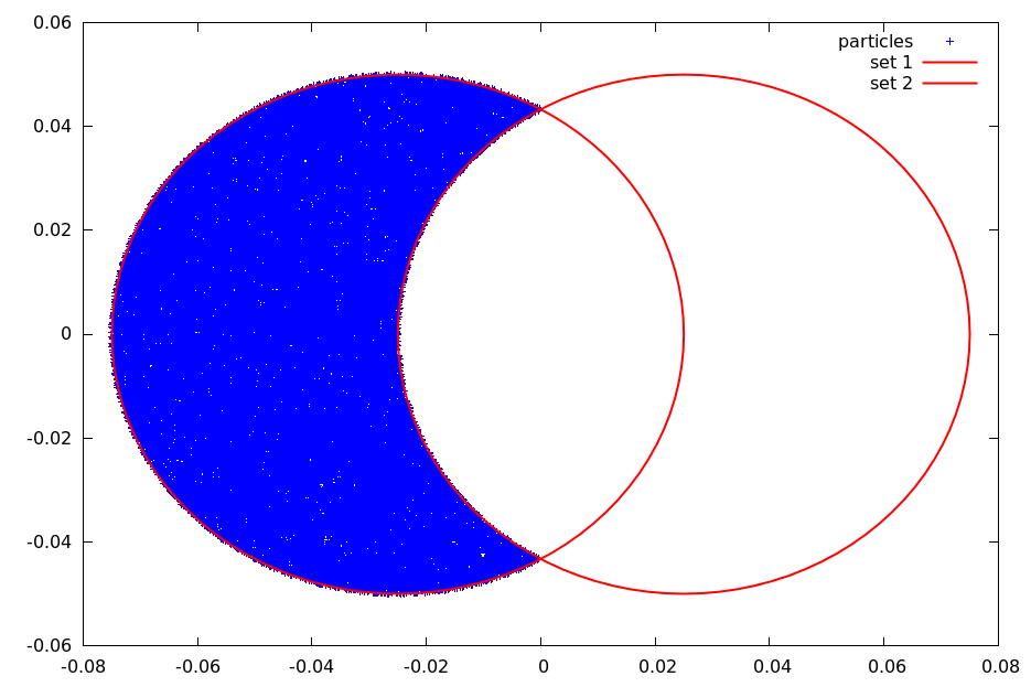
- symmetric_difference(command1, command2)
-
All particles that pass either command but not both at the same time.
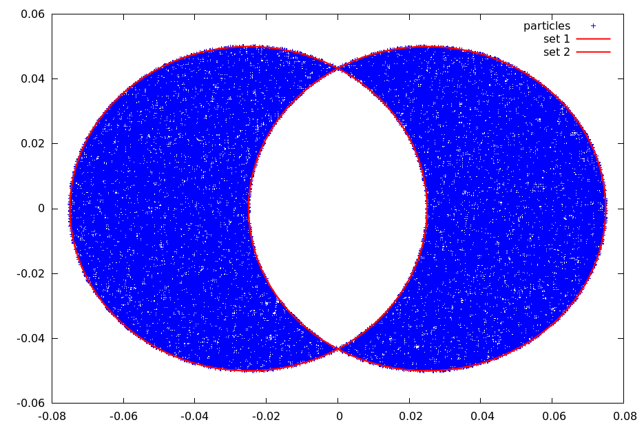
- intersection(command1, command2)
-
All particles that pass both commands at the same time.
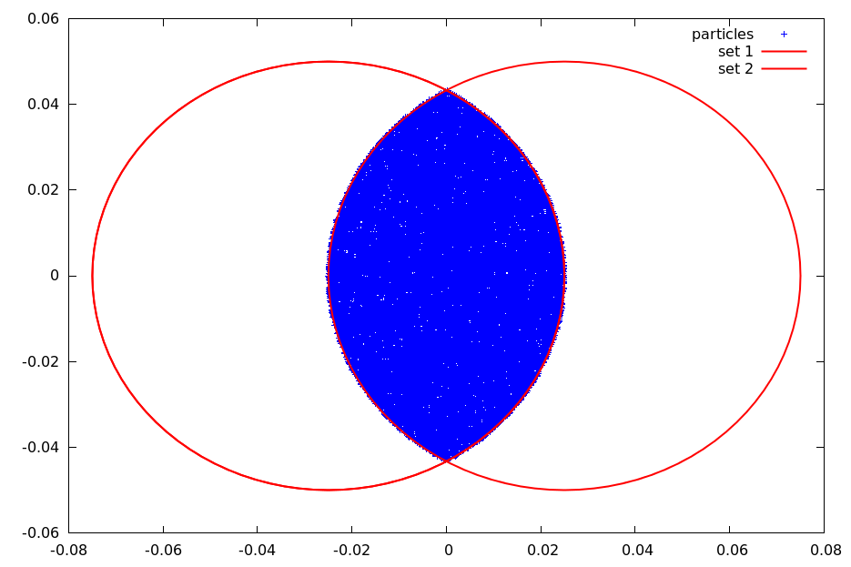
- repeat(command, N, shiftx, shifty)
-
Repeats the holes that are defined by the command translating each copy successively by shiftx in x-direction and shifty in y-direction. The arguments shiftx and shifty can be mathematical expressions.
- repeat(command, N, angle)
-
Repeats the holes that are defined by the command rotating each copy successively. The argument angle can be a mathematical expression.
The supported mathematical constants and functions are listed in the following table.
e |
pi |
abs(x) |
acos(x) |
acosh(x) |
asin(x) |
asinh(x) |
atan(x) |
atanh(x) |
cbrt(x) |
ceil(x) |
cos(x) |
cosh(x) |
deg2rad(x) |
erf(x) |
erfc(x) |
exp(x) |
exp2(x) |
floor(x) |
isinf(x) |
isnan(x) |
log(x) |
log2(x) |
log10(x) |
rad2deg(x) |
round(x) |
sgn(x) |
sin(x) |
sinh(x) |
sqrt(x) |
tan(x) |
tanh(x) |
tgamma(x) |
atan2(y,x) |
max(x,y) |
min(x,y) |
A simple elliptic collimator with major and minor axis of 4 cm and 3 cm respectively can be defined using
ellipse(0.04, 0.03)
A regular pepper-pot with rectangular holes can be define like this
repeat( // repeat it in y-direction
       repeat( // repeat it in x-direction
              translate(
                        rotate(
                               rectangle(
                                         0.002,
                                         0.002
                                        ),
                               0.78539
                              ),
                        -0.028,
                        -0.028
                       ),
              16,
              0.004,
              0.0
             ),
       16,
       0.0,
       0.004
      )
The latter example will produce a holes as in the following picture
In the FLEXIBLECOLLIMATOR command the description of the holes can be provided as a string (using DESCRIPTION; the string may not contain comments and newlines) or in a separate file (using FNAME; comments and newlines are allowed).
11.19.2. OPAL-cycl mode
Only CCOLLIMATOR is available for OPAL-cycl. This element is radial
rectangular collimator which can be used to collimate the radial tail
particles. When a particle hits this collimator, it will be absorbed
or scattered. The algorithm is based on the Monte Carlo method. Please
note when a particle is scattered, it will not be recorded as the lost
particle. If this particle leaves the bunch, it will be removed during
the integration afterwards, so as to maintain the accuracy of space
charge solving. In addition to the general attributes of a collimator
(OUTFN and PARTICLEMATTERINTERACTION), the parameters for describing a
CCOLLIMATOR are the following:
- XSTART
-
The x coordinate of the start point. [mm]
- XEND
-
The x coordinate of the end point. [mm]
- YSTART
-
The y coordinate of the start point. [mm]
- YEND
-
The y coordinate of the end point. [mm]
- ZSTART
-
The minimum vertical coordinate [mm]. Default value is -100mm.
- ZEND
-
The maximum vertical coordinate. [mm]. Default value is 100mm.
- WIDTH
-
The width of the collimator. [mm]
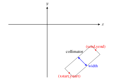
Example:
REAL y1=-0.0;
REAL y2=0.0;
REAL y3=200.0;
REAL y4=205.0;
REAL x1=-215.0;
REAL x2=-220.0;
REAL x3=0.0;
REAL x4=0.0;

cmphys: PARTICLEMATTERINTERACTION, TYPE=SCATTERING, MATERIAL="Copper";

cma1: CCollimator, XSTART=x1, XEND=x2,YSTART=y1, YEND=y2,
      ZSTART=2, ZEND=100, WIDTH=10.0, PARTICLEMATTERINTERACTION=cmphys ;

cma2: CCollimator, XSTART=x3, XEND=x4,YSTART=y3, YEND=y4,
      ZSTART=2, ZEND=100, WIDTH=10.0, PARTICLEMATTERINTERACTION=cmphys;
The particles lost on the CCOLLIMATOR are recorded in the HDF5 file
OUTFN.h5 (or ASCII if ASCIIDUMP is true).
11.20. Septum (OPAL-cycl)
This is a restricted feature for OPAL-cycl. The particles hitting on the
septum are removed from the bunch and recorded in the OUTFN file.
There are 5 parameters to describe a septum.
- XSTART
-
The x coordinate of the start point. [mm]
- XEND
-
The x coordinate of the end point. [mm]
- YSTART
-
The y coordinate of the start point. [mm]
- YEND
-
The y coordinate of the end point. [mm]
- WIDTH
-
The width of the septum. [mm]
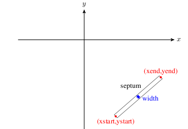
Example:
eec2: Septum, xstart=4100.0, xend=4300.0,
ystart=-1200.0, yend=-150.0, width=0.05;
The particles lost on the SEPTUM are recorded in the HDF5 file
OUTFN.h5 (or ASCII if ASCIIDUMP is true).
11.21. Probe (OPAL-cycl)
The particles hitting on the probe are recorded in the OUTFN file
(see Common Attributes).
There are 5 parameters to describe a probe.
- XSTART
-
The x coordinate of the start point. [mm]
- XEND
-
The x coordinate of the end point. [mm]
- YSTART
-
The y coordinate of the start point. [mm]
- YEND
-
The y coordinate of the end point. [mm]
- STEP
-
The step size of the probe (for histogram and peak finder output). Default: 1 [mm]
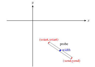
Example:
prob1: Probe, xstart=4166.16, xend=4250.0,
ystart=-1226.85, yend=-1241.3;
The particles probed on the PROBE are recorded in the HDF5 file
OUTFN.h5 (or ASCII if ASCIIDUMP is true).
Please note that these particles are not deleted
in the simulation, however, they are recorded in the "loss" file.
The radius of the particles recorded in the PROBE is recorded in the histogram ".hist" and peak ".peaks" file. The histogram file contains data as recorded in actual probe measurements. The corresponding peaks file contains the peaks found in the probe histogram by the same peak finder used for the PSI measurements. Note that for probes in multiple quadrants the histogram and peaks file is often not meaningful since the absolute radius is stored.
11.22. Stripper (OPAL-cycl)
A stripper element strip the electron(s) from a particle. The particle
hitting the stripper is recorded in the OUTFN file
(see Common Attributes), which contains
the time, coordinates and momentum of the particle at the moment it hit
the stripper. The charge and mass are changed. It has the same geometry as
the PROBE element. Please note that the stripping physics is not
included yet.
There are 9 parameters to describe a stripper.
- XSTART
-
The x coordinate of the start point. [mm]
- XEND
-
The x coordinate of the end point. [mm]
- YSTART
-
The y coordinate of the start point. [mm]
- YEND
-
The y coordinate of the end point. [mm]
- OPCHARGE
-
Charge number of the outcoming particle. Negative value represents negative charge.
- OPMASS
-
Mass of the outcoming particles. [\(\mathrm{GeV/c^2}\)]
- OPYIELD
-
Yield of the outcoming particle (the number of outcoming particles per incoming particle), the default value is 1.
- STOP
-
If STOP is true, the particle is stopped and deleted from the simulation; Otherwise, the outcoming particle continues to be tracked along the extraction path.
Example: \(H_2^+\) particle stripping
prob1: Stripper, xstart=4166.16, xend=4250.0,
ystart=-1226.85, yend=-1241.3,
opcharge=1, opmass=PMASS, opyield=2, stop=false;
No matter what the value of STOP is, the particles hitting on the
STRIPPER are recorded in the HDF5 file
OUTFN.h5 (or ASCII if ASCIIDUMP is true).
11.23. Degrader (OPAL-t)
Elliptical degrader with an overall length L. The particles
lost on a degrader are recorded in the OUTFN file
(see Common Attributes).
- XSIZE
-
Major axis of the transverse elliptical shape, default value is 1e6.
- YSIZE
-
Minor axis of the transverse elliptical shape, default value is 1e6.
- PARTICLEMATTERINTERACTION
-
PARTICLEMATTERINTERACTIONis an attribute of the element (see Chapter Particle Matter Interaction).TYPE=SCATTERINGmust be selected to include scattering interactions and energy loss calculation through theMATERIALdefinition (see Available Materials in OPAL). If this is not set, the particle-matter interaction module will not be activated. The particle hitting degrader will be recorded and directly deleted from the simulation.
Example: Graphite degrader of 15 cm thickness.
DEGPHYS: PARTICLEMATTERINTERACTION, TYPE=SCATTERING, MATERIAL="Graphite";

DEG1: DEGRADER, L=0.15, ELEMEDGE=0.02, PARTICLEMATTERINTERACTION=DEGPHYS;
11.24. Correctors (OPAL-t)
Three types of correctors are available:
- HKICKER
-
A corrector for the horizontal plane.
- VKICKER
-
A corrector for the vertical plane.
- KICKER
-
A corrector for both planes.
They act as
label:HKICKER, TYPE=string, APERTURE=real-vector,
      L=real, KICK=real;
label:VKICKER, TYPE=string, APERTURE=real-vector,
      L=real, KICK=real;
label:KICKER, TYPE=string, APERTURE=real-vector,
      L=real, HKICK=real, VKICK=real;
They have the following attributes:
- L
-
The length of the closed orbit corrector (default: 0 m).
- KICK
-
The kick angle in rad for either horizontal or vertical correctors (default: 0 rad).
- HKICK
-
The horizontal kick angle in rad for a corrector in both planes (default: 0 rad).
- VKICK
-
The vertical kick angle in rad for a corrector in both planes (default: 0 rad).
- DESIGNENERGY
-
Fix the magnitude of the magnetic field using the given
DESIGNENERGYand the angle (KICK,HKICKorVKICK). If the design energy isn’t set then the actual energy of the reference particle at the position of the corrector is used. TheDESIGNENERGYis expected in MeV.
A positive kick increases \(p_{x}\) or \(p_{y}\)
respectively. Use KICK for an HKICKER or VKICKER and HKICK and
VKICK for a KICKER. Instead of using a KICKER or a VKICKER one
could use an HKICKER and rotate it appropriately using PSI.
Correctors don’t change the reference trajectory. Otherwise they are
implemented as RBEND with \(\mathrm{E1} = 0\) and without
fringe fields (hard edge model). They can be used to model earth’s
magnetic field which is neglected in the design trajectory but which has
a noticeable effect on the trajectory of a bunch at low energies.
Examples:
HK1:HKICKER, KICK=0.001;
VK3:VKICKER, KICK=0.0005;
KHV:KICKER, HKICK=0.001, VKICK=0.0005;
The reference system for an orbit corrector is a Cartesian coordinate system.
11.25. Vacuum (OPAL-cycl)
Vacuum element represents the conditions and parameters to consider interactions with the residual gas and the magnetic field in a cyclotron. When the particle interacts, it is recorded in the file, which contains the time, coordinates and momentum of the particle at this moment. The particle could produce a new particle, changing the charge and mass.
There are 7 parameters to describe the vacuum space.
- PRESSURE
-
The average pressure of the residual gas in the cyclotron. [mbar]
- TEMPERATURE
-
Temperature of residual gas. [K]
- PMAPFN
-
File name of the mid-plane pressure map. The pressure data is stored in a sequence shown in 2D field map on the median plane with primary direction corresponding to the azimuthal direction, secondary direction to the radial direction (same file structure as
CyclotronTYPE=CARBONCYCL). IfPMAPFNis specified,PRESSUREparameter is taken as default value for regions in the accelerator out of the limits of the pressure map. - PSCALE
-
Scale factor for the pressure field map (default: 1.0).
- GAS
-
Type of gas for residual vacuum:
H2orAIR - STOP
-
If STOP is true, the particle is stopped and deleted from the simulation. Otherwise, the outcoming particle continues to be tracked as
SECONDARYparticle (default: true). - PARTICLEMATTERINTERACTION
-
PARTICLEMATTERINTERACTIONis an attribute of the element (see Chapter Particle Matter Interaction).TYPE=BEAMSTRIPPINGmust be selected to include stripping interactions with the residual gas and Lorentz stripping.
Example: Vacuum representation with \(H_2\) residual gas.
bstp_phys: PARTICLEMATTERINTERACTION, TYPE=BEAMSTRIPPING;

vac: VACUUM, PRESSURE=1E-8, TEMPERATURE=300,
      GAS="H2", STOP=true, PARTICLEMATTERINTERACTION=bstp_phys;
No matter what the value of STOP is, the particles stripped are recorded in the HDF5 file
(or ASCII if ASCIIDUMP is true).
11.26. Undulator (OPAL-t)
OPAL's undulator element comes with its own Finite-Difference Time-Domain full-wave solver, which accounts for space-charge and radiation effects in 3D. It was implemented by means of the MITHRA library, developed by Arya Fallahi.
To use the undulator element and its solver, one needs to compile OPAL in the following way:
-
install the MITHRA 2.0 library,
-
set the environment variable
MITHRA_PREFIX=directory/where/you/store/mithra -
compile OPAL with the option
cmake -DENABLE_OPAL_FEL=yes ..
When the head of the bunch crosses the start of an undulator in the beamline
(defined by ELEMEDGE), the solver changes automatically from
Poisson to full-wave, and changes back to Poisson once the bunch has passed through the
whole undulator and its fringe fields.
The length of the undulator is defined as
where \(\lambda\) is the undulator period and \(N\) its number of periods.
Since the element’s length is entirely defined by the undulator periods, there is no LENGTH
parameter to be specified for the undulator element.
The magnetic field is that of a planar undulator with flat pole faces:
where \(r = x\cos(\alpha) + y\sin(\alpha)\) is the radial distance from the undulator axis, \(k=2\pi/\lambda\) the wave-number, \(\alpha\) the angle between the magnetic field polarisation and the x-axis, and \(B_0\) the maximum magnetic field value.
The fringe fields are defined as:
The parameters that describe the undulator element and its associated full-wave solver are as follows:
- K
-
The undulator strength parameter.
- LAMBDA
-
The undulator period \(\lambda\) [m].
- NUMPERIODS
-
Number of periods \(N\).
- ANGLE
-
Angle \(\alpha\) between the magnetic field polarisation and the x-axis [rad] (default: 0).
- MESHLENGTH
-
Size in three dimensions \((L_x, L_y, L_z)\) of the computational grid [m], which is in a frame of reference moving at the average speed of the bunch. It should be large enough to contain the whole bunch, as particles outside of it will not perceive any fields. As a rule of thumb, the grid should be 3 times longer than the bunch, since the bunch will slightly shift longitudinally when entering and exiting the undulator, and 10 times wider than the bunch, to avoid spurious radiation reflections, since the Absorbing Boundary Conditions (ABCs) cannot correctly absorb obliquely incident waves.
- MESHRESOLUTION
-
Grid-spacing \((\Delta_x, \Delta_y, \Delta_z)\) of the computational domain [m].
- DTBUNCH
-
Time-step for the particle update [s]. By default it is equal to the field update time-step, which is automatically chosen by the algorithm in order to satisfy the stability conditon.
DTBUNCHneeds to be equal to or smaller than the field time-step. - TRUNORDER
-
Truncation order of the ABCs. Can be 1 or 2 (default: 2).
- TOTALTIME
-
Total time to simulate using the full-wave solver [s]. By default this is set such that the whole passage through the undulator is simulated.
- FNAME
-
File specifying which output the full-wave solver should provide. It is equivalent to the job-file in MITHRA, without the parameters
MESH,bunch-initialization, andUNDULATOR. This file is optional.
Example of the wiggler element used in the AWA beamline:
UND: UNDULATOR, ELEMEDGE = 44.0e-2, K = 10.81, LAMBDA = 8.5e-2, NUMPERIODS = 10, ANGLE = PI/2,
     MESHLENGTH = { 12e-3, 12e-3, 4e-3 }, MESHRESOLUTION = { 1e-5, 1e-5, 8e-6},
     FNAME = "wiggler_sims_July_2020/mithra_output.job";
11.27. References
[24] J. E. Spencer and H. A. Enge, Split-pole magnetic spectrograph for precision nuclear spectroscopy, Nucl. Instrum. Methods 49, 181 (1967).
12. Field Output
There are two routines that can be used to write out the external field used in OPAL-cycl.
- DUMPFIELDS
-
write out static magnetic field map on a Cartesian grid
- DUMPEMFIELDS
-
write out electromagnetic field map on a 4D grid in space-time. Cartesian and cylindrical grids are supported.
DUMPEMFIELDSis an extension ofDUMPFIELDS.
12.1. DUMPFIELDS Command
The DUMPFIELDS statement causes OPAL-cycl to write out static magnetic field data on a 3D cartesian grid. The format of field output is:
<number of rows>
1 x [m]
2 y [m]
3 z [m]
4 Bx [kGauss]
5 By [kGauss]
6 Bz [kGauss]
0
<x0> <y0> <z0> <Bx0> <By0> <Bz0>
<x1> <y1> <z1> <Bx1> <By1> <Bz1>
...
The following attributes are enabled on the DUMPFIELDS statement:
- FILE_NAME
-
Name of the file to which field data is dumped. It is an error if the location reference by
FILE_NAMEcannot be opened. Any existing file is overwritten. - X_START
-
Start point in the grid in x [m]
- DX
-
Grid step size in x [m]
- X_STEPS
-
Number of steps in x. It is an error if
X_STEPSis non-integer or less than 1. - Y_START
-
Start point in the grid in y [m]
- DY
-
Grid step size in y [m]
- Y_STEPS
-
Number of steps in y. It is an error if
Y_STEPSis non-integer or less than 1. - Z_START
-
Start point in the grid in z [m]
- DZ
-
Grid step size in z [m]
- Z_STEPS
-
Number of steps in z. It is an error if
Z_STEPSis non-integer or less than 1.
This example makes a field map in the midplane (x-y plane) only, starting at \((x,y) = (0,0)\) m, with 101 steps in each direction and a stride of 0.1 m. z is always 0.
DUMPFIELDS, X_START=0., X_STEPS=101, DX=0.100,
            Y_START=0., Y_STEPS=101, DY=0.100,
            Z_START=0., Z_STEPS=1, DZ=0.100,
            FILE_NAME="FieldMapXY.dat";
12.2. DUMPEMFIELDS Command
The DUMPEMFIELDS statement causes OPAL-cycl to write out electromagnetic field data on a 4D grid. Grids in a Cartesian coordinate system \((x,y,z,t)\) and a cylindrical coordinate system about the z-axis in \((r,\phi,z,t)\) are supported.
12.2.1. Cartesian Mode
In Cartesian mode the format of the field output is:
<number of rows>
1 x [m]
2 y [m]
3 z [m]
4 t [ns]
5 Bx [kGauss]
6 By [kGauss]
7 Bz [kGauss]
8 Ex [?]
9 Ey [?]
10 Ez [?]
0
<x0> <y0> <z0> <t0> <Bx0> <By0> <Bz0> <Ex0> <Ey0> <Ez0>
<x1> <y1> <z1> <t1> <Bx1> <By1> <Bz1> <Ex1> <Ey1> <Ez1>
...
The following attributes are enabled on the DUMPEMFIELDS statement when operating in Cartesian mode:
- FILE_NAME
-
Name of the file to which field data is dumped. It is an error if the location referenced by
FILE_NAMEcannot be opened. Any existing file is overwritten. - COORDINATE_SYSTEM
-
Either 'Cartesian' or 'Cylindrical'. The string is not case sensitive. It is an error if the string is not one of 'cartesian' or 'cylindrical'.
- X_START
-
Start point in the grid in x
- DX
-
Grid step size in x
- X_STEPS
-
Number of steps in x. It is an error if
X_STEPSis non-integer or less than 1. - Y_START
-
Start point in the grid in y
- DY
-
Grid step size in y
- Y_STEPS
-
Number of steps in y. It is an error if
Y_STEPSis non-integer or less than 1. - Z_START
-
Start point in the grid in z
- DZ
-
Grid step size in z.
- Z_STEPS
-
Number of steps in z. It is an error if
Z_STEPSis non-integer or less than 1. - T_START
-
Start point in the grid in time
- DT
-
Grid step size in time.
- T_STEPS
-
Number of steps in time. It is an error if
T_STEPSis non-integer or less than 1.
12.2.2. Cylindrical Mode
In Cylindrical mode the format of the field output is:
<number of rows>
1 r [m]
2 phi [degree]
3 z [m]
4 t [ns]
5 Br [kGauss]
6 Bphi [kGauss]
7 Bz [kGauss]
8 Er [MV/m]
9 Ephi [MV/m]
10 Ez [MV/m]
0
<r0> <phi0> <z0> <t0> <Br0> <Bphi0> <Bz0> <Er0> <Ephi0> <Ez0>
<r1> <phi1> <z1> <t1> <Br1> <Bphi1> <Bz1> <Er1> <Ephi1> <Ez1>
...
The following attributes are enabled on the DUMPEMFIELDS statement when operating in Cylindrical mode:
- FILE_NAME
-
Name of the file to which field data is dumped. It is an error if the location referenced by
FILE_NAMEcannot be opened. Any existing file is overwritten. - COORDINATE_SYSTEM
-
Either 'Cartesian' or 'Cylindrical'. The string is not case sensitive. It is an error if the string is not one of 'cartesian' or 'cylindrical'.
- R_START
-
Start point in the grid in r [m]
- DR
-
Grid step size in r [m]
- R_STEPS
-
Number of steps in r. It is an error if
R_STEPSis non-integer or less than 1. - PHI_START
-
Start point in the grid in phi [rad]
- DPHI
-
Grid step size in phi [rad]
- PHI_STEPS
-
Number of steps in phi. It is an error if
PHI_STEPSis non-integer or less than 1. - Z_START
-
Start point in the grid in z [m]
- DZ
-
Grid step size in z [m]
- Z_STEPS
-
Number of steps in z. It is an error if
Z_STEPSis non-integer or less than 1. - T_START
-
Start point in the grid in time [ns]
- DT
-
Grid step size in time [ns]
- T_STEPS
-
Number of steps in time. It is an error if
T_STEPSis non-integer or less than 1.
13. Beam Lines
The accelerator to be studied is known to OPAL as a sequence of
physical elements called a beam line. A beam line is built from
simpler beam lines whose definitions can be nested to any level. A
powerful syntax allows to repeat or to reflect pieces of beam lines.
Formally a beam line is defined by a LINE command:
label:LINE=(member,...,member);
label gives a name to the beam line for later reference.
Each member may be one of the following:
-
An element label,
-
A beam line label,
-
A sub-line, enclosed in parentheses,
Beam lines can be nested to any level.
13.1. Simple Beam Lines
The simplest beam line consists of single elements:
label:LINE=(member,...,member);
Example:
L:LINE=(A,B,C,D,A,D);
- ORIGIN
-
Position vector of the origin of the line. All elements in this line that are placed using
ELEMEDGEuse this position as reference. - ORIENTATION
-
Vector of Tait-Bryan angles [bib.tait-bryan] of the orientation of the line at the origin.
13.2. Sub-lines
Instead of referring to an element, a beam line member can refer to another beam line defined in a separate command. This provides a shorthand notation for sub-lines which occur several times in a beam line. Lines and sub-lines can be entered in any order, but when a line is used, all its sub-lines must be known.
Example:
 L:LINE=(A,B,S,B,A,S,A,B);
 S:LINE=(C,D,E);
This example produces the following expansion steps:
-
Replace sub-line
S:(A,B,(C,D,E),B,A,(C,D,E),A,B)
-
Omit parentheses:
A,B,C,D,E,B,A,C,D,E,A,B
evaluated to constants immediately.
14. Beam Command
All OPAL commands working on a beam require the setting of various
quantities related to this beam. These are entered by a BEAM command:
label:BEAM, PARTICLE=name, MASS=real, CHARGE=real,
      ENERGY=real, PC=real, GAMMA=real, BCURRENT=real,
      NPART=real, BFREQ=real;
The label is optional, it defaults to UNNAMED_BEAM.
14.1. Particle Definition
The particle mass and charge are defined by:
- PARTICLE
-
The name of particles in the machine.
OPAL knows the mass (see Predefined Symbolic Constants) and the charge for the following particles:
- POSITRON
-
The particles are positrons (
MASS= \(m_e\),CHARGE= 1). - ELECTRON
-
The particles are electrons (
MASS= \(m_e\),CHARGE= -1). - PROTON
-
The particles are protons (default,
MASS= \(m_p\),CHARGE= 1). - ANTIPROTON
-
The particles are anti-protons (
MASS= \(m_p\),CHARGE= -1). - HMINUS
-
The particles are negative hydrogen ions (H-) (
MASS= \(m_{hm}\),CHARGE= -1). - CARBON
-
The particles are carbons (
MASS= \(m_c\),CHARGE= 12). - URANIUM
-
The particles are of type uranium (
MASS= \(m_u\),CHARGE= 35). - MUON
-
The particles are of type muon (
MASS= \(m_\mu\),CHARGE= -1). - DEUTERON
-
The particles are of type deuteron (
MASS= \(m_d\),CHARGE= 1). - XENON
-
The particles are of type xenon (
MASS= \(m_{xe}\),CHARGE= 20). - H2P
-
The particles are of type molecular hydrogen ions+ (
MASS= \(m_{h2p}\),CHARGE= 1). - ALPHA
-
The particles are of alpha particles (
MASS= \(m_{\alpha}\),CHARGE= 2).
For other particle names one may enter:
- MASS
-
The particle mass in GeV.
- CHARGE
-
The particle charge expressed in elementary charges.
14.2. Beam Energy
To specify the energy there are three attributes (in order of priority):
- GAMMA
-
The particle energy divided by its mass.
- ENERGY
-
The particle energy in GeV.
- PC
-
The particle momentum in GeV/c.
14.3. Other Attributes
The other attributes are:
- BFREQ
-
The bunch frequency in MHz.
- BCURRENT
-
The bunch current in A. \(\mathrm{BCURRENT} = Q \times \mathrm{BFREQ}\) with \(Q\) the total charge.
- NPART
-
The number of macro particles for the simulations
- NSLICE
-
The number of slices per bunch
15. Distribution Command
| Distribution Type | Description |
|---|---|
Initial distribution read in from text file provided by user. |
|
Initial distribution generated using Gaussian distribution(s). |
|
Initial distribution generated using flattop distribution(s). |
|
Initial distribution generated using binomial distribution(s). |
|
Initial distribution generated using matched Gaussian distribution(s). |
|
Legacy. Special case of |
|
Legacy. Special case of |
The distribution command is used to introduce particles into an OPAL simulation. Like other OPAL commands see Chapter Command Format, the distribution command is of the form:
Name:DISTRIBUTION, TYPE = DISTRIBUTION_TYPE,
                   ATTRIBUTE #1 =,
                   ATTRIBUTE #2 =,
                   .
                   .
                   .
                   ATTRIBUTE #N =;
The distribution is given a name (which is used to reference the distribution in the OPAL input file), a distribution type, and a list of attributes. The types of distributions that are supported are listed in Table 15. The attributes that follow the distribution type further define the particle distribution. Some attributes are universal, while others are specific to the distribution type. In the following sections we will define the distribution attributes, starting with the general, or universal attributes. (Note that, in general, if a distribution type does not support a particular attribute, defining a value for it does no harm. That attribute just gets ignored.)
15.1. Units
The internal units used by OPAL-t and OPAL-cycl are described in
OPAL-t variables and OPAL-cycl variables.
When defining a
distribution, both OPAL-t and OPAL-cycl use meters for length and
seconds for time. However, there are different options for the units
used to input the momentum. This is controlled with the
INPUTMOUNITS attribute.
| Attribute Name | Value | Description |
|---|---|---|
|
|
Use no units for the input momentum (\(p_{x}\), \(p_{y}\), \(p_{z}\)). Momentum is given as \(\beta_{x} \gamma\), \(\beta_{y} \gamma\) and \(\beta_{z} \gamma\), as in OPAL-t variables. |
|
|
Use the units eV/c for the input momentum (\(p_{x}\), \(p_{y}\), \(p_{z}\)). |
15.2. note: unit conversion of momentum in OPAL-t and OPAL-cycl
Convert \(\beta_x \gamma\) [dimensionless] to [mrad],
Convert from [eV/c] to \(\beta_x\gamma\) [dimensionless],
This may be deduced by analogy for the \(y\) and \(z\) directions.
15.3. General Distribution Attributes
Once the distribution type is chosen, the next attribute to specify is
the EMITTED attribute.
The EMITTED attribute controls whether a distribution is injected or
emitted. An injected distribution is placed in its entirety into the
simulation space at the start of the simulation. An emitted beam is
emitted into the simulation over time as the simulation progresses (e.g.
from a cathode in a photoinjector simulation). Currently, only OPAL-t
supports emitted distributions. The default is an injected
distribution.
| Attribute Name | Value | Description |
|---|---|---|
|
|
The distribution is injected into the simulation in its entirety at the start of the simulation. The particle coordinates for an injected distribution are defined as in OPAL-t variables and OPAL-cycl variables. Note that in OPAL-t the entire distribution will automatically be shifted to ensure that the \(z\) coordinate will be greater than zero for all particles. |
|
|
The distribution is emitted into the simulation over time as the simulation progresses. Currently only OPAL-t supports this type of distribution. In this case, the longitudinal coordinate, as defined by OPAL-t variables, is given in seconds instead of meters. Early times are emitted first. |
Depending on the EMITTED attribute, we can specify several other
attributes that do not depend on the distribution type. These are
defined in
Universal Attributes, Injected Distribution Attributes and Emitted Distribution Attributes.
15.3.1. Universal Attributes
| Attribute Name | Default Value | Units | Description |
|---|---|---|---|
|
|
None |
Echo initial distribution to text file data/<basename > DIST.dat_. |
|
|
None |
Makes the generation scalable with respect of number of particles. The result depends on the number of cores used. |
|
1.0 |
None |
Weight of distribution when used in a distribution list see Distribution List. |
|
0 |
None |
The distribution (beam) will be broken up into |
|
100 |
None |
Number of sample bins to use per energy bin. |
|
1.0 |
None |
Value used to scale the \(x\) positions of the distribution particles. Applied after the distribution is generated (or read in). |
|
1.0 |
None |
Value used to scale the \(y\) positions of the distribution particles. Applied after the distribution is generated (or read in). |
|
1.0 |
None |
Value used to scale the x momentum, \(p_{x}\), of the distribution particles. Applied after the distribution is generated (or read in). |
|
1.0 |
None |
Value used to scale the y momentum, \(p_{y}\), of the distribution particles. Applied after the distribution is generated (or read in). |
|
1.0 |
None |
Value use to scale the z momentum, \(p_{z}\), of the distribution particles. Applied after the distribution is generated (or read in). |
|
0.0 |
m |
Distribution is shifted in \(x\) by this amount after the distribution is generated (or read in). Same as the average \(x\) position, \(\bar{x}\). |
|
0.0 |
m |
Distribution is shifted in \(y\) by this amount after the distribution is generated (or read in). Same as the average \(y\) position, \(\bar{y}\). |
|
0.0 |
Distribution is shifted in \(p_{x}\) by this amount after the distribution is generated (or read in). Same as the average \(p_{x}\) value, \(\bar{p}_{x}\). |
|
|
0.0 |
Distribution is shifted in \(p_{y}\) by this amount after the distribution is generated (or read in). Same as the average \(p_{y}\) value, \(\bar{p}_{y}\). |
|
|
0.0 |
Distribution is shifted in \(p_{z}\) by this amount after the distribution is generated (or read in). Same as the average \(p_{z}\) value, \(\bar{p}_{z}\). |
|
|
{0.0, 0.0, 0.0, 0.0, 0.0, 0.0} |
Tracer particle which is written also into data/track_orbit.dat. Expects an array with 6 items, \(x,\; y,\; z,\; p_x,\; p_y,\; p_z\). Not supported in OPAL-t. |
|
|
{0.0, 0.0, 0.0, 0.0, 0.0, 0.0} |
Tracer particle which is written also into data/track_orbit.dat. Expects an array with 6 items, \(x,\; y,\; z,\; p_x,\; p_y,\; p_z\). Not supported in OPAL-t. |
15.3.2. Injected Distribution Attributes
| Attribute Name | Default Value | Units | Description |
|---|---|---|---|
|
1.0 |
None |
Value used to scale the \(z\) positions of the distribution particles. Applied after the distribution is generated (or read in). |
|
0.0 |
m |
Distribution is shifted in \(z\) by this
amount relative to the reference particle. Same as the average
\(z\) position, \(\bar{z}\). To shift the position
where the particles are injected please use |
15.3.3. Emitted Distribution Attributes
| Attribute Name | Default Value | Units | Description |
|---|---|---|---|
|
1.0 |
None |
Value used to scale the \(t\) values of the distribution particles. Applied after the distribution is generated (or read in). |
|
0.0 |
s |
Distribution is emitted later by this amount relative to the reference particle. |
|
1 |
None |
Number of time steps to take during emission. The simulation time step will be adjusted during emission to ensure that this many time steps will be required to emit the entire distribution. |
|
None |
None |
Emission model to use when emitting particles from cathode see Emission Models. |
15.4. FROMFILE Distribution Type
The most versatile distribution type is to use a user generated text file as input to OPAL. This allows the user to generate their own distribution, if the built in options in OPAL are insufficient, and have it either injected or emitted into the simulation. In Table 21 we list the single attribute specific to this type of distribution type.
| Attribute Name | Default Value | Units | Description |
|---|---|---|---|
|
None |
None |
File name for text file containing distribution particle coordinates. |
An example of an injected FROMFILE distribution definition is:
Name:DISTRIBUTION, TYPE = FROMFILE,
                   FNAME = "text file name";
an example of an emitted FROMFILE distribution definition is:
Name:DISTRIBUTION, TYPE = FROMFILE,
                   FNAME = "text file name",
                   EMITTED = TRUE,
                   EMISSIONMODEL = None;
The text input file for the FROMFILE distribution type has a
slightly different format, depending on whether the distribution is to
be injected or emitted. The injected file format is defined in
Table 22. The particle coordinates are defined in OPAL-t variables and OPAL-cycl variables. The emitted file format is defined in
Table 23. The particle coordinates are defined in OPAL-t variables except that \(z\), in meters, is replaced by \(t\) in seconds.
N |
|||||
\(x_{1}\) |
\(p_{x1}\) |
\(y_{1}\) |
\(p_{y1}\) |
\(z_{1}\) |
\(p_{z1}\) |
\(x_{2}\) |
\(p_{x2}\) |
\(y_{2}\) |
\(p_{y2}\) |
\(z_{2}\) |
\(p_{z2}\) |
. |
|||||
. |
|||||
\(x_{N}\) |
\(p_{xN}\) |
\(y_{N}\) |
\(p_{yN}\) |
\(z_{N}\) |
\(p_{zN}\) |
N |
|||||
\(x_{1}\) |
\(p_{x1}\) |
\(y_{1}\) |
\(p_{y1}\) |
\(t_{1}\) |
\(p_{z1}\) |
\(x_{2}\) |
\(p_{x2}\) |
\(y_{2}\) |
\(p_{y2}\) |
\(t_{2}\) |
\(p_{z2}\) |
. |
|||||
. |
|||||
\(x_{N}\) |
\(p_{xN}\) |
\(y_{N}\) |
\(p_{yN}\) |
\(t_{N}\) |
\(p_{zN}\) |
Note that for an emitted FROMFILE distribution, all of the
particle’s time, \(t\), coordinates will be shifted to
negative time (if they are not there already). The simulation clock will
then start at \(t = 0\) and distribution particles will be
emitted into the simulation as the simulation progresses. Also note
that, as the particles are emitted, they will be modified according to
the type of emission model used. This is defined by the attribute
EMISSIONMODEL, which is described in Emission Models. A choice
of NONE for the EMISSIONMODEL (which is the default) can be defined
so as not to affect the distribution coordinates at all.
To maintain consistency \(N\) and NPART from the BEAM
command in Chapter Beam Command must be equal.
15.5. GAUSS Distribution Type
As the name implies, the GAUSS distribution type can generate
distributions with a general Gaussian shape (here we show a
one-dimensional example):
where \(\bar{x}\) is the average value of \(x\).
However, the GAUSS distribution can also be used to generate an
emitted beam with a flat top time profile. We will go over the various
options for the GAUSS distribution type in this section.
15.5.1. Simple GAUSS Distribution Type
We will begin by describing how to create a simple GAUSS distribution
type. That is, a simple 6-dimensional distribution with a Gaussian
distribution in all dimensions.
| Attribute Name | Default Value | Units | Description |
|---|---|---|---|
|
0.0 |
m |
RMS width, \(\sigma_{x}\), in transverse \(x\) direction. |
|
0.0 |
m |
RMS width, \(\sigma_{y}\), in transverse \(y\) direction. |
|
0.0 |
m |
RMS radius, \(\sigma_{r}\), in radial
direction. If nonzero |
|
0.0 |
m or s |
RMS length, \(\sigma_{z}\), of the Gaussian
in longitudinal (z) direction. |
|
0.0 |
m or s |
RMS length, \(\sigma_{t}\), of the Gaussian
in longitudinal (z) direction. |
|
0.0 |
Parameter \(\sigma_{px}\) for defining distribution. |
|
|
0.0 |
Parameter \(\sigma_{py}\) for defining distribution. |
|
|
0.0 |
Parameter \(\sigma_{pz}\) for defining distribution. |
|
|
3.0 |
None |
Defines transverse distribution cutoff in the
\(x\) direction in units of \(\sigma_{x}\). If
|
|
3.0 |
None |
Defines transverse distribution cutoff in the
\(y\) direction in units of \(\sigma_{y}\). If
|
|
3.0 |
None |
Defines transverse distribution cutoff in the
\(r\) direction in units of \(\sigma_{r}\). If
|
|
3.0 |
None |
Defines longitudinal distribution cutoff in
the \(z\) or \(t\) direction (injected or
emitted) in units of \(\sigma_{z}\) or
\(\sigma_{t}\). |
|
3.0 |
None |
Defines cutoff in \(p_{x}\) dimension
in units of \(\sigma_{px}\). If |
|
3.0 |
None |
Defines cutoff in \(p_{y}\) dimension
in units of \(\sigma_{py}\). If |
|
3.0 |
None |
Defines cutoff in \(p_{z}\) dimension
in units of \(\sigma_{pz}\). If |
In Table 24 we list the basic attributes available for a
GAUSS distribution. We can use these to create a very simple GAUSS
distribution:
Name:DISTRIBUTION, TYPE       = GAUSS,
                   SIGMAX     = 0.001,
                   SIGMAY     = 0.003,
                   SIGMAZ     = 0.002,
                   SIGMAPX    = 0.0,
                   SIGMAPY    = 0.0,
                   SIGMAPZ    = 0.0,
                   CUTOFFX    = 2.0,
                   CUTOFFY    = 2.0,
                   CUTOFFLONG = 4.0,
                   OFFSETX    = 0.001,
                   OFFSETY    = -0.002,
                   OFFSETZ    = 0.01,
                   OFFSETPZ   = 1200.0;
This creates a Gaussian shaped distribution with zero transverse emittance, zero energy spread, \(\sigma_{x} = {1.0} \mathrm{mm}\), \(\sigma_{y} = {3.0} \mathrm{mm}\), \(\sigma_{z} = {2.0} \mathrm{mm}\) and an average energy of:
In the \(x\) direction, the Gaussian distribution is cutoff at \(x = 2.0 \times \sigma_{x} = {2.0} \mathrm{mm}\). In the \(y\) direction it is cutoff at \(y = 2.0 \times \sigma_{y} = {6.0} \mathrm{mm}\). This distribution is injected into the simulation at an average position of \((\bar{x},\bar{y},\bar{z})=({1.0} \mathrm{mm}, {-2.0} \mathrm{mm}, {10.0} \mathrm{mm})\).
15.5.2. GAUSS Distribution for Photoinjector
| Attribute Name | Default Value | Units | Description |
|---|---|---|---|
|
0.0 |
s |
Flat top time see Figure 29. |
|
0.0 |
s |
Rise time see Figure 29. If defined will
override |
|
0.0 |
s |
Fall time see Figure 29. If defined will
override |
|
0 |
None |
Sinusoidal oscillations can imposed on the flat top in Figure 29. This defines the amplitude of those oscillations in percent of the average flat top amplitude. |
|
0 |
None |
Defines the number of oscillation periods imposed on the flat top, \(t_\mathrm{flattop}\), in Figure 29. |
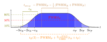
GAUSS distribution with flat top.A useful feature of the GAUSS distribution type is the ability to
mimic the initial distribution from a photoinjector. For this purpose we
have the distribution attributes listed in Table 25.
Using them, we can create a distribution with the time structure shown
in Figure 29. This is a half Gaussian rise plus a uniform
flat-top plus a half Gaussian fall. To make it more convenient to mimic
measured laser profiles, TRISE and TFALL from
Table 25 do not define RMS quantities, but instead
are given by (See also Figure 29):
where \(\sigma_{R}\) and \(\sigma_{F}\) are the
Gaussian, RMS rise and fall times respectively. The flat-top portion of
the profile, TPULSEFWHM, is defined as (See also Figure 29):
Total emission time, \(t_{E}\), of this distribution, is a
function of the longitudinal cutoff, CUTOFFLONG
see Table 24, and is given by:
Finally, we can also impose oscillations over the flat-top portion of
the laser pulse in Figure 29, \(t_\mathrm{flattop}\).
This is defined by the attributes FTOSCAMPLITUDE and FTOSCPERIODS
from Table 25. FTOSCPERIODS defines how many
oscillation periods will be present during the
\(t_\mathrm{flattop}\) portion of the pulse. FTOSCAMPLITUDE
defines the amplitude of those oscillations in percentage of the average
profile amplitude during \(t_\mathrm{flattop}\). So, for
example, if we set \(\mathrm{FTOSCAMPLITUDE} = 5\), and the
amplitude of the profile is equal to \(1.0\) during
\(t_\mathrm{flattop}\), the amplitude of the oscillation will
be \(0.05\).
15.5.3. Correlations for GAUSS Distribution (Experimental)
| Attribute Name | Default Value | Units | Description |
|---|---|---|---|
|
All 15 correlations in a single array (\(R_{12}, R_{13}, .. , R_{56}\)). |
||
|
0.0 |
\(x\), \(p_x\) correlation. (\(R_{12}\) in transport notation.) |
|
|
0.0 |
\(y\), \(p_y\) correlation. (\(R_{34}\) in transport notation.) |
|
|
0.0 |
\(z\), \(p_z\) correlation. (\(R_{56}\) in transport notation.) |
|
|
0.0 |
same as and overwritten by |
|
|
0.0 |
\(x\), \(z\) correlation. (\(R_{51}\) in transport notation.) |
|
|
0.0 |
\(p_x\), \(z\) correlation. (\(R_{52}\) in transport notation.) |
|
|
0.0 |
\(x\), \(p_z\) correlation. (\(R_{61}\) in transport notation.) |
|
|
0.0 |
\(p_x\), \(p_z\) correlation. (\(R_{62}\) in transport notation.) |
To generate Gaussian initial distribution with dispersion, first we generate the uncorrelated Gaussian inputs matrix \(R=(R_1,...,R_n)\). The mean of \(R_i\) is \(0\) and the standard deviation squared is 1. Then we correlate \(R\). The correlation coefficient matrix \(\sigma\) in \(x\), \(p_x\), \(z\), \(p_z\) phase space reads:
The Cholesky decomposition of the symmetric positive-definite matrix \(\sigma\) is \(\sigma=C^{\mathbf{T}}C\), then the correlated distribution is \(C^{\mathbf{T}}R\).
Note: Correlations work for the moment only with the Gaussian distribution and are experimental, so there are no guarantees as to its efficacy or accuracy. Also, these correlations will work, in principle, for an emitted beam. However, recall that in this case, \(z\) in meters is replaced by \(t\) in seconds, so take care.
As an example of defining a correlated beam, let the initial correlation coefficient matrix be:
then the corresponding distribution command will read:
Dist:DISTRIBUTION, TYPE = GAUSS,
                   SIGMAX = 4.796e-03,
                   SIGMAPX = 231.0585,
                   CORRX = 0.756,
                   SIGMAY = 23.821e-03,
                   SIGMAPY = 1.6592e+03,
                   CORRY = -0.999,
                   SIGMAZ = 0.466e-02,
                   SIGMAPZ = 74.7,
                   CORRZ = -0.834,
                   OFFSETZ = 0.466e-02,
                   OFFSETPZ = 72e6,
                   R61 = 0.496,
                   R62 = -0.042,
                   R51 = 0.023,
                   R52 = 0.385;
15.6. FLATTOP Distribution Type
The FLATTOP distribution type is used to define hard edge beam
distributions. Hard edge, in this case, means a more or less uniformly
filled cylinder of charge, although as we will see this is not always
the case. The main purpose of the FLATTOP is to mimic laser pulses in
photoinjectors, and so we usually will make this an emitted
distribution. However it can be injected as well.
15.6.1. Injected FLATTOP
The attributes for an injected FLATTOP distribution are defined in
Table 27 and Table 18. At the moment, we cannot
define a spread in the beam momentum, so an injected FLATTOP
distribution will currently have zero emittance. An injected FLATTOP
will be a uniformly filled ellipse transversely with a uniform
distribution in \(z\). (Basically a cylinder with an
elliptical cross section.)
| Attribute Name | Default Value | Units | Description |
|---|---|---|---|
|
0.0 |
m |
Hard edge width in \(x\) direction. |
|
0.0 |
m |
Hard edge width in \(y\) direction. |
|
0.0 |
m |
Hard edge radius. If nonzero |
|
0.0 |
m |
Hard edge length in \(z\) direction. |
15.6.2. Emitted FLATTOP
| Attribute Name | Default Value | Units | Description |
|---|---|---|---|
|
0.0 |
m |
Hard edge width in \(x\) direction. |
|
0.0 |
m |
Hard edge width in \(y\) direction. |
|
0.0 |
m |
Hard edge radius. If nonzero |
|
0.0 |
s |
RMS rise and fall of half Gaussian in flat top defined in in Figure 29. |
|
0.0 |
s |
Flat top time. See Figure 29. |
|
0.0 |
s |
Rise time. See Figure 29. If defined will
override |
|
0.0 |
s |
Fall time. See Figure 29. If defined will
override |
|
0 |
None |
Sinusoidal oscillations can imposed on the flat top in Figure 29. This defines the amplitude of those oscillations in percent of the average flat top amplitude. |
|
0 |
None |
Defines the number of oscillation periods imposed on the flat top, \(t_\mathrm{flattop}\), in Figure 29. |
|
None |
File name containing measured laser image. |
|
|
None |
Used for h5 files. Name of the groups containing the laser image, see regression test. |
|
|
0.0 |
None |
Parameter defining floor of the background to be subtracted from the laser image in percent of the maximum intensity. |
|
|
Flip the laser profile in horizontal direction. |
|
|
|
Flip the laser profile in vertical direction. |
|
|
|
Rotate the laser profile 90\(^{\circ}\) in counterclockwise direction. |
|
|
|
Rotate the laser profile 180\(^{\circ}\). |
|
|
|
Rotate the laser profile 270\(^{\circ}\) in counterclockwise direction. |
The attributes of an emitted FLATTOP distribution are defined in
Table 28 and Table 18. The FLATTOP
distribution was really intended for this mode of operation in order to
mimic common laser pulses in photoinjectors. The basic characteristic of
a FLATTOP is a uniform, elliptical transverse distribution and a
longitudinal (time) distribution with a Gaussian rise and fall time as
described in GAUSS Distribution for Photoinjector. Below we show an
example of a FLATTOP distribution command with an elliptical cross
section of 1 mm by 2 mm and a flat top, in time, 10 ps long with a 0.5 ps
rise and fall time as defined in Figure 29.
Dist:DISTRIBUTION, TYPE = FLATTOP,
                   SIGMAX = 0.001,
                   SIGMAY = 0.002,
                   TRISE = 0.5e-12,
                   TFALL = 0.5e-12,
                   TPULSEFWHM = 10.0e-12,
                   CUTOFFLONG = 4.0,
                   NBIN = 5,
                   EMISSIONSTEPS = 100,
                   EMISSIONMODEL = ASTRA,
                   EKIN = 0.5,
                   EMITTED = TRUE;
15.6.3. Transverse Distribution from Laser Profile (Under Development)
An alternative to using a uniform, elliptical transverse profile is to
define the LASERPROFFN, IMAGENAME and INTENSITYCUT attributes from
Table 28. Then, OPAL-t will use the laser image as
the basis to sample the transverse distribution.
This distribution option is not yet available.
15.6.4. GUNGAUSSFLATTOPTH Distribution Type
This is a legacy distribution type. A GUNGAUSSFLATTOPTH is the
equivalent of a FLATTOP distribution, except that the EMITTED
attribute will set to TRUE automatically and the EMISSIONMODEL will
be automatically set to ASTRA.
15.6.5. ASTRAFLATTOPTH Distribution Type
This is a legacy distribution type. A ASTRAFLATTOPTH is the equivalent
of a FLATTOP distribution, except that the EMITTED attribute will
set to TRUE automatically and the EMISSIONMODEL will be
automatically set to ASTRA. There are a few other differences with how
the longitudinal time profile of the distribution is generated.
15.7. BINOMIAL Distribution Type
The BINOMIAL type of distribution is based on [25]. The shape of
the binomial distribution is governed by one parameter \(m\).
By varying this single parameter one obtains the most commonly used
distributions for our type of simulations, as listed in
Table 29 and shown in Figure 30.
| \(m\) | Distribution | Density | Profile |
|---|---|---|---|
0.0 |
Hollow shell |
\(\frac{1}{\pi}\delta(1-r^2)\) |
\(\frac{1}{\pi}(1-x^2)^{-0.5}\) |
0.5 |
Flat profile |
\(\frac{1}{2\pi}(1-r^2)^{-0.5}\) |
\(\frac{1}{2}\) |
1.0 |
Uniform |
\(\frac{1}{\pi}\) |
\(\frac{2}{\pi}(1-x^2)^{0.5}\) |
1.5 |
Elliptical |
\(\frac{3}{2\pi}(1-r^2)^{0.5}\) |
\(\frac{1}{4}(1-x^2)\) |
2.0 |
Parabolic |
\(\frac{2}{\pi}(1-r^2)\) |
\(\frac{3}{8\pi}(1-x^2)^{1.5}\) |
\(\rightarrow \infty (> 10000)\) |
Gaussian |
\(\frac{1}{2\pi\sigma_x\sigma_y}exp(-\frac{x^2}{2\sigma_x^2} -\frac{y^2}{2\sigma_y^2})\) |
\(\frac{1}{\sqrt{2\pi} \sigma_x}exp(-\frac{x^2}{2\sigma_x^2}) \) |
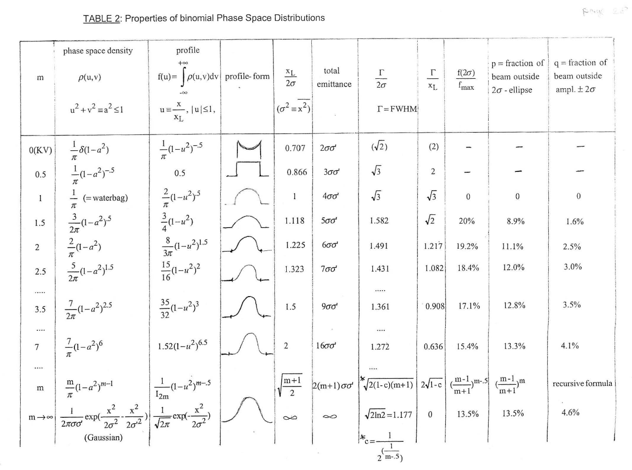
The attributes of a BINOMIAL distribution are defined in Table 30.
| Attribute Name | Default Value | Units | Description |
|---|---|---|---|
|
10001 |
Defines parameter \(m\) for the binomial distribution in \(x\) |
|
|
10001 |
Defines parameter \(m\) for the binomial distribution in \(y\) |
|
|
10001 |
Defines parameter \(m\) for the binomial distribution in \(z\) |
|
|
10001 |
Same as and overwritten by |
The width and the (\(x,p_x\)) phase space is given by the usual SIGMAX (\(\sigma_x\)),
SIGMAXP (\(\sigma_{xp}\)) and CORRX (\(\sigma_{12}\))
and defined as follows (similarly for the other dimensions):
Example:
Dist:DISTRIBUTION, TYPE    = BINOMIAL,
                   SIGMAX  = 2.15e-03,
                   SIGMAPX = 1E-6,
                   CORRX   = 0.0,
                   MX      = 0.01,
                   SIGMAY  = 0.50*23.e-03,
                   SIGMAPY = 28.0,
                   CORRY   = 0.5,
                   MY      = 990.0,
                   SIGMAT  = 1.0e-1,
                   SIGMAPT = 11.96,
                   CORRT   = -0.5,
                   MT      = 2.0,
15.8. GAUSSMATCHED Matched Gauss Distribution type
The attributes of a GAUSSMATCHED distribution are defined in 31.
Limitation: Does not consider Trimcoil field maps!
| Attribute Name | Default Value | Units | Description |
|---|---|---|---|
|
1E-3 |
GeV |
Energy step size for closed orbit finder |
|
1E-6 |
m rad |
Projected normalized emittance in \(x\) |
|
1E-6 |
m rad |
Projected normalized emittance in \(y\) |
|
1E-6 |
m rad |
Projected normalized emittance in \(t\) |
|
720 |
Number of integration steps of closed orbit finder |
|
|
1 |
Number of sectors to average field for closed orbit finder |
|
|
TRUE |
Match using single sector (true) or all sectors (false) |
|
|
7 |
Order used in the field expansion |
|
|
-1 |
Guess value of radius (m) for closed orbit finder |
|
|
1E-8 |
Residuum for the closed orbit finder and sigma matrix generator |
|
|
100 |
Maximum steps used to find closed orbit |
|
|
500 |
Maximum steps used to find matched distribution |
15.9. MULTIGAUSS Distribution type
The purpose of this distribution is to mimic photoinjectors in which the laser beam consists of a train of Gaussian pulses [26]. Therefore this distribution has a uniform elliptical transverse distribution, and a train of equally spaced normal distributions along the z or t axis.
This distribution can be emitted or injected. When emitted, each particle acquires momentum according to the emission model. When injected, the momentum follows a normal distribution, and the user can specify \( (\sigma_{px}, \sigma_{py}, \sigma_{pz})\).
| Attribute Name | Default Value | Units | Description |
|---|---|---|---|
|
0.0 |
m |
Laser radius in transverse \(x\) direction. |
|
0.0 |
m |
Laser radius in transverse \(y\) direction. |
|
0.0 |
m |
Laser radius, \(\sigma_{r}\), in radial
direction. If nonzero |
|
0.0 |
m or s |
RMS length of each Gaussian pulse
in longitudinal (z) direction. |
|
0.0 |
m or s |
RMS length of each Gaussian pulse
in longitudinal (z) direction. |
|
0.0 |
m or s |
Peak-to-peak distance between the Gaussian pulses in longitudinal (z) direction. Use seconds for an emitted bunch, and meters for an injected one. |
|
1 |
None |
Number of pulses along the longitudinal (z) direction. |
|
3.0 |
None |
Cutoff distance from the center of the
first and last Gaussian pulses in the \(z\) or
\(t\) direction (injected or emitted) in units of
\(\sigma_{z}\) or \(\sigma_{t}\). |
|
0.0 |
Parameter \(\sigma_{px}\) for the normal distribution of the momentum. This parameter is ignored for an emitted bunch. |
|
|
0.0 |
Parameter \(\sigma_{py}\) for the normal distribution of the momentum. This parameter is ignored for an emitted bunch. |
|
|
0.0 |
Parameter \(\sigma_{pz}\) for the normal distribution of the momentum. This parameter is ignored for an emitted bunch. |
|
|
3.0 |
None |
Defines cutoff in \(p_{x}\) dimension
in units of \(\sigma_{px}\). If |
|
3.0 |
None |
Defines cutoff in \(p_{y}\) dimension
in units of \(\sigma_{py}\). If |
|
3.0 |
None |
Defines cutoff in \(p_{z}\) dimension
in units of \(\sigma_{pz}\). If |
In 32 the basic attributes available for a
MULTIGAUSS distribution are listed.
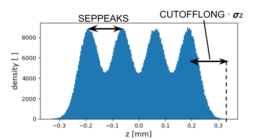
MULTIGAUSS distribution.An example (fig. 31) of a MULTIGAUSS injected bunch could be:
Dist: DISTRIBUTION, TYPE = MULTIGAUSS,
                    SIGMAPX = 1e-2, SIGMAPY = 1e-2, SIGMAPZ = 1e-2,  // In units of betaGamma
                    CUTOFFPX = 4.0, CUTOFFPY = 4.0, CUTOFFPZ = 4.0,  // In units of SIGMAP
                    SIGMAR = 340e-6,
                    SIGMAZ = 90e-6 / 2.355, // FWHM  = 2.355 * sigma
                    CUTOFFLONG = 4.0,  // In units of SIGMAZ
                    SEPPEAKS = 126e-6,
                    NPEAKS = 4,
                    EMITTED = FALSE;
15.10. Emission Models
When emitting a distribution from a cathode, there are several ways in which we can model the emission process in order to calculate the thermal emittance of the beam. In this section we discuss the various options available.
15.10.1. Emission Model: NONE (default)
The emission model NONE is the default emission model used in
OPAL-t. It has a single attribute, listed in
Table 33. The NONE emission model is very
simplistic. It merely adds the amount of energy defined by the attribute
EKIN to the longitudinal momentum, \(p_{z}\), for each
particle in the distribution as it leaves the cathode.
| Attribute Name | Default Value | Units | Description |
|---|---|---|---|
|
1.0 |
eV |
Thermal energy added to beam during emission. |
An example of using the NONE emission model is given below. This
option allows us to emit transversely cold (zero x and y emittance)
beams into our simulation. We must add some z momentum to ensure that
the particles drift into the simulation space. If in this example one
were to specify EKIN = 0, then you would likely get strange results as
the particles would not move off the cathode, causing all of the emitted
charge to pile up at \(z = 0\) in the first half time step
before the beam space charge is calculated.
Dist:DISTRIBUTION, TYPE = FLATTOP,
                   SIGMAX = 0.001,
                   SIGMAY = 0.002,
                   TRISE = 0.5e-12,
                   TFALL = 0.5e-12,
                   TPULSEFWHM = 10.0e-12,
                   CUTOFFLONG = 4.0,
                   NBIN = 5,
                   EMISSIONSTEPS = 100,
                   EMISSIONMODEL = NONE,
                   EKIN = 0.5,
                   EMITTED = TRUE;
One thing to note, it may be that if you are emitting your own
distribution using the TYPE = FROMFILE option, you may want to set
EKIN = 0 if you have already added some amount of momentum,
\(p_{z}\), to the particles.
15.10.2. Emission Model: ASTRA
The ASTRA emittance model uses the same single parameter as the NONE
option as listed in Table 33. However, in this
case, the energy defined by the EKIN attribute is added to each
emitted particle’s momentum in a random way:
where \(\theta\) is a random angle between \(0\) and \(\pi\), and \(\phi\) is given by
with \(x\) a random number between \(0\) and \(1\).
15.10.3. Emission Model: NONEQUIL
The NONEQUIL emission model is based on an actual physical model of
particle emission as described in [27], [28], [29]. The
attributes needed by this emission model are listed in
Table 34.
| Attribute Name | Default Value | Units | Description |
|---|---|---|---|
|
4.86 |
eV |
Photoinjector drive laser energy. (Default is 255nm light.) |
|
4.31 |
eV |
Photocathode work function. (Default is atomically clean copper.) |
|
7.0 |
eV |
Fermi energy of photocathode. (Default is atomically clean copper.) |
|
300.0 |
K |
Operating temperature of photocathode. |
An example of using the NONEQUIL emission model is given below. This
model is relevant for metal cathodes and cathodes such as CsTe.
Dist:DISTRIBUTION, TYPE = GAUSS,
                   SIGMAX = 0.001,
                   SIGMAY = 0.002,
                   TRISE = 1.0e-12,
                   TFALL = 1.0e-12,
                   TPULSEFWHM = 15.0e-12,
                   CUTOFFLONG = 3.0,
                   NBIN = 10,
                   EMISSIONSTEPS = 100,
                   EMISSIONMODEL = NONEQUIL,
                   ELASER = 6.48,
                   W = 4.1,
                   FE = 7.0,
                   CATHTEMP = 325,
                   EMITTED = TRUE;
15.10.4. Distribution List
It is possible to use multiple distributions in the same simulation. We
do this be using a distribution list in the RUN command
see Chapter Tracking. Assume we have defined several distributions:
DIST1, DIST2 and DIST3. If we want to use just one of these
distributions in a simulation, we would use the following RUN command
to start the simulation:
RUN, METHOD = "PARALLEL-T",
     BEAM = beam_name,
     FIELDSOLVER = field_solver_name,
     DISTRIBUTION = DIST1;
If we want to use all the distributions at the same time, then the command would instead be:
RUN, METHOD = "PARALLEL-T",
     BEAM = beam_name,
     FIELDSOLVER = field_solver_name,
     DISTRIBUTION = {DIST1, DIST2, DIST3};
In this second case, the first distribution (DIST1) is the master
distribution. The main consequence of this is that all distributions in
the list will be forced to the same EMITTED condition as DIST1. So,
if DIST1 is to be emitted, then all other distributions in the list
will be forced to this same condition. If DIST1 is to be injected,
then all other distribution is the list will also be injected.
The number of particles in the simulation is defined in the BEAM
command see Chapter Beam Command. The number of particles in each distribution
in a distribution list is determined by this number and the WEIGHT
attribute of each distribution (Table 18). If all
distributions have the same WEIGHT value, then the number of particles
will be divided up evenly among them. If, however we have a distribution
list consisting of two distributions, and one has twice the WEIGHT of
the other, then it will have twice the particles as its partner. The
exception here is any FROMFILE distribution type. In this case, the
WEIGHT attribute and the number of particles in the BEAM command are
ignored. The number of particles in any FROMFILE distribution type is
defined by the text file containing the distribution particle
coordinates. (FROMFILE Distribution Type).
15.11. References
[25] W. Joho, Representation of beam ellipses for transport calculations, PSI Internal Report TM-11-14, Paul Scherrer Institute (1980).
[26] J. G. Power and C. Jing, Temporal Laser Pulse Shaping for RF Photocathode Guns: The Cheap and Easy way using UV Birefringent Crystals, AIP Conf. Proc. 1086, 689 (2009).
[27] K. Flöttmann, Note on the thermal emittance of electrons emitted by Cesium Telluride photo cathodes, Tech. Rep. DESY-TESLA-FEL-97-01, Deutsches Elektronen-Synchrotron (1997).
[28] J. E. Clendenin et al., Reduction of thermal emittance of RF guns, Nucl. Instrum. Methods A 455, 198 (2000).
[29] D. H. Dowell and J. F. Schmerge, Quantum efficiency and thermal emittance of metal photocathodes, Phys. Rev. ST Accel. Beams 12, 074201 (2009).
16. Field Solver
Space charge effects are included in the simulation by specifying a field solver described in this chapter and attaching it to the track command as described in Chapter Tracking. By default, the code does not assume any symmetry i.e. full 3D. In the near future it is planed to implement also a slice (2D) model. This will allow the use of less numbers of macro-particles in the simulation which reduces the computational time significantly.
The space charge forces are calculated by solving the 3D Poisson equation with open boundary conditions using a standard or integrated Green function method. The image charge effects of the conducting cathode are also included using a shifted Green function method. If more than one Lorentz frame is defined, the total space charge forces are then the summation of contributions from all Lorentz frames. More details will be given in Version 2.0.0.
16.1. FFT Based Particle-Mesh (PM) Solver
The Particle-Mesh (PM) solver is one of the oldest improvements over the PP solver. Still one of the best references is the book by R.W. Hockney & J.W. Eastwood [30]. The PM solver introduces a discretization of space. The rectangular computation domain \(\Omega:=[-L_x,L_x]\times[-L_y,L_y]\times[-L_t,L_t]\), just big enough to include all particles, is segmented into a regular mesh of \(M=M_x\times M_y\times M_t\) grid points. For the discussion below we assume \(N=M_x=M_y=M_t\).
The solution of Poisson’s equation is an essential component of any self-consistent electrostatic beam dynamics code that models the transport of intense charged particle beams in accelerators. If the bunch is small compared to the transverse size of the beam pipe, the conducting walls are usually neglected. In such cases the Hockney method may be employed [30], [31] and [32]. In that method, rather than computing \(N_p^2\) point-to-point interactions (where \(N_p\) is the number of macro-particles), the potential is instead calculated on a grid of size \((2 N)^d\), where \(N\) is the number of grid points in each dimension of the physical mesh containing the charge, and where \(d\) is the dimension of the problem. Using the Hockney method, the calculation is performed using Fast Fourier Transform (FFT) techniques, with the computational effort scaling as \((2N)^d (log_2 2N)^d\).
When the beam bunch fills a substantial portion of the beam pipe transversely, or when the bunch length is long compared with the pipe transverse size, the conducting boundaries cannot be ignored. Poisson solvers have been developed previously to treat a bunch of charge in an open-ended pipe with various geometries [33] , [34].
The solution of the Poisson equation,
for the scalar potential, \(\phi\), due to a charge density, \(\rho\), and appropriate boundary conditions, can be expressed as,
where \(G(x,x',y,y',z,z')\) is the Green function, subject to the appropriate boundary conditions, describing the contribution of a source charge at location \((x',y',z')\) to the potential at an observation location \((x,y,z)\).
For an isolated distribution of charge this reduces to
where
A simple discretization of Convolution solution on a Cartesian grid with cell size \((h_x,h_y,h_z)\) leads to,
where \(\rho_{i,j,k}\) and \(G_{i-i',j-j',k-k'}\) denote the values of the charge density and the Green function, respectively, defined on the grid \(M\).
16.1.1. FFT-based Convolutions and Zero Padding
FFTs can be used to compute convolutions by appropriate zero-padding of the sequences. Discrete convolutions arise in solving the Poisson equation, and one is typically interested in the following,
where \(\bar{G}\) corresponds to the free space Green function, \(\bar{\rho}\) corresponds to the charge density, and \(\bar{\phi}\) corresponds to the scalar potential. The sequence \(\{\bar{\phi}_j\}\) has \(J\) elements, \(\{\bar{\rho}_k\}\) has \(K\) elements, and \(\{\bar{G}_m\}\) has \(M=J+K-1\) elements.
One can zero-pad the sequences to a length \(N\ge M\) and use FFT’s to efficiently obtain the \(\{\bar{\phi}_j\}\) in the unpadded region. This defines a zero-padded charge density, \(\rho\),
Define a periodic Green function, \(G_m\), as follows,
Now consider the sum
where \(W=e^{-2\pi i/N}\). This is just the FFT-based convolution of \(\{\rho_k\}\) with \(\{G_m\}\). Then,
Now use the relation
It follows that
But \(G\) is periodic with period \(N\). Hence,
In the physical (unpadded) region, \(j\in \left[0,J-1\right]\), so the quantity \(j-n\) in Final equation satisfies \(-(K-1)\le j-n \le J-1\). In other words the values of \(G_{j-n}\) are identical to \(\bar{G}_{j-n}\). Hence, in the physical region the FFT-based convolution, FFT convolution, matches the convolution in Brute force convolution.
As stated above, the zero-padded sequences need to have a length \(N \ge M\), where \(M\) is the number of elements in the Green function sequence \(\left\{x_m\right\}\). In particular, one can choose \(N=M\), in which case the Green function sequence is not padded at all, and only the charge density sequence, \(\left\{r_k\right\}\), is zero-padded, with \(k=0,\ldots,K-1\) corresponding to the physical region and \(k=K,\ldots,M-1\) corresponding to the zero-padded region.
The above FFT-based approach – zero-padding the charge density array, and circular-shifting the Green function in accordance with Periodic Green function – will work in general. In addition, if the Green function is a symmetric function of its arguments, the value at the end of the Green function array (at grid point \(J-1\)) can be dropped, since it will be recovered implicitly through the symmetry of Periodic Green function. In that case the approach is identical to the Hockney method [30], [31] and [32]. Lastly, note that the above proof that the convolution, FFT convolution, is identical to Brute force convolution in the unpadded region, works even when \(W^{-j k}\) and \(W^{m k}\) are replaced by \(W^{j k}\) and \(W^{-m k}\), respectively, in FFT convolution. In other words, the FFT-based approach can be used to compute
simply by changing the direction of the Fourier transform of the Green function and changing the direction of the final Fourier transform.
16.1.2. Algorithm used in OPAL
As a result, the solution of Open brute force convolution is then given by
where the notation has been introduced that \(\text{FFT}\{ . \}\) denotes a forward FFT in all 3 dimensions, and \(\text{FFT}^{-1}\{ . \}\) denotes a backward FFT in all 3 dimensions.
16.1.3. Interpolation Schemes
More details will be given in Version 2.0.0.
16.2. Iterative Space Charge Solver
This is a scalable parallel solver for the Poisson equation within a Particle-In-Cell (PIC) code for the simulation of electron beams in particle accelerators of irregular shape. The problem is discretized by Finite Differences. Depending on the treatment of the Dirichlet boundary the resulting system of equations is symmetric or `mildly' non-symmetric positive definite. In all cases, the system is solved by the preconditioned conjugate gradient algorithm with smoothed aggregation (SA) based algebraic multigrid (AMG) preconditioning. More details are given in [35].
This solver is enabled with ENABLE_SAAMG_SOLVER=ON in the OPAL compilation.
It requires Parmetis and Trilinos to be installed.
16.3. Energy Binning
The beam out of a cathode or in a plasma wake field accelerator can have a large energy spread. In this case, the static approximation using one Lorentz frame might not be sufficient. Multiple Lorentz frames can be used so that within each Lorentz frame the energy spread is small and hence the electrostatic approximation is valid. More details will be given in Version 2.0.0.
16.4. The FIELDSOLVER Command
See Table 35 for a summary of the Fieldsolver command.
| Command | Purpose |
|---|---|
|
Specify a fieldsolver |
|
Specify the type of field solver: |
|
If |
|
If |
|
If |
|
Number of grid points in \(x\) specifying rectangular grid |
|
Number of grid points in \(y\) specifying rectangular grid |
|
Number of grid points in \(z\) specifying rectangular grid |
|
Boundary condition in \(x\) [ |
|
Boundary condition in \(y\) [ |
|
Boundary condition in \(z\) [ |
|
Defines the Greens function for the FFT Solver. ( |
|
Enlargement of the bounding box in % |
|
Geometry to be used as domain boundary. ( |
|
Type of iterative solver. ( |
|
Interpolation used for boundary points. ( |
|
Tolerance for iterative solver. ( |
|
Maximum number of iterations of iterative solver. ( |
|
Behavior of the preconditioner. ( |
16.5. Define the Fieldsolver to be used
At present FFT based solver is the most stable solver. Other solvers include Finite Element solvers and a Multigrid solver with Shortley-Weller boundary conditions for irregular domains.
16.6. Define Domain Decomposition
The dimensions in \(x\), \(y\) and \(z\)
can be parallel (TRUE) or serial FALSE. The default settings are:
parallel in \(z\) and serial in \(x\) and
\(y\).
16.7. Define Number of Grid Points
Number of grid points in \(x\), \(y\) and \(z\) for a rectangular grid.
16.8. Define Boundary Conditions
Two boundary conditions can be selected independently among
\(x\), \(y\) namely: OPEN and for \(z\)
OPEN & PERIODIC. In the case you select for \(z\) periodic
you are about to model a DC-beam.
16.9. Define Greens Function
16.10. Define Bounding Box Enlargement
The bounding box defines a minimal rectangular domain including all
particles. With BBOXINCR the bounding box can be enlarged by a factor
given in percent of the minimal rectangular domain. Default value is 2.0.
16.11. Define Geometry
The list of geometries defining the beam line boundary. For further details see Chapter Geometry.
16.12. Define Iterative Solver
The iterative solver for solving the preconditioned system: CG (default),
BICGSTAB or GMRES.
16.13. Define Interpolation for Boundary Points
The interpolation method for grid points near the boundary: CONSTANT,
LINEAR (default) or QUADRATIC.
16.14. Define Tolerance
The tolerance for the iterative solver used by the SAAMG solver.
Default value is 1e-8.
16.15. Define Maximal Iterations
The maximal number of iterations the iterative solver performs. Default value is 100.
16.16. Define Preconditioner Behavior
The behavior of the preconditioner can be: STD, HIERARCHY or
REUSE. This argument is only relevant when using the SAAMG solver and
should only be set if the consequences to simulation and solver are
evident. A short description is given in the
Table below.
| Value | Behavior |
|---|---|
|
The preconditioner is rebuilt in every time step |
|
The hierarchy (tentative prolongator) is reused (enabled by default) |
|
The preconditioner is reused |
16.17. Define the number of Energy Bins to use
Suppose \(\mathrm{d} E\) the energy spread in the particle
bunch is to large, the electrostatic approximation is no longer valid.
One solution to that problem is to introduce \(k\) energy bins
and perform \(k\) separate field solves in which
\(\mathrm{d} E\) is again small and hence the electrostatic
approximation valid. In case of a cyclotron see Cyclotron the
number of energy bins must be at minimum the number of neighboring
bunches (NNEIGHBB) i.e.
\(\mathrm{ENBINS} \le \mathrm{NNEIGHBB}\).
The variable MINSTEPFORREBIN defines the number of integration step
that have to pass until all energy bins are merged into one.
16.18. Define AMR Solver
After compiling OPAL with ENABLE_AMR=ON, the option AMR=TRUE enables further
commands to be used in the Fieldsolver command (cf. Table 37).
The current AMR interface in OPAL is based on AMReX [39] which provides the
multigrid solvers FMG (till release 18.07) and ML. We also provide a Trilinos based solver
which is described in the section Hardware-Architecture Independent AMR Poisson Solver.
In order to setup an AMR simulation, the user has to specify the number of AMR levels. The
hierarchy is built based on the values of the refinement ratios, blocking factors and
maximum grid sizes of the base level. The maximum grid size of the next higher level is
given by the division with the refinement ratio. The same is true for
the blocking factors. The mesh refinement follows user-dependent rules that are
provided by AMR_TAGGING. The various mesh refinement methods are provided in
Table 38.
| Command | Purpose |
|---|---|
|
AMR Poisson solvers: |
|
Maximum adaptive mesh refinement level (single level if
|
|
Grid cell refinement ratio in x, only |
|
Grid cell refinement ratio in y, only |
|
Grid cell refinement ratio in z, only |
|
Maximum grid size of base level in x. It has to be smaller than
|
|
Maximum grid size of base level in y. It has to be smaller than
|
|
Maximum grid size of base level in z. It has to be smaller than
|
|
AMReX blocking factor in x. |
|
AMReX blocking factor in y. |
|
AMReX blocking factor in z. |
|
Mesh-refinement strategy [ |
|
Charge density refinement threshold when |
|
Refinement threshold for |
|
Refinement threshold for |
|
Refinement threshold for |
|
Box ratio of the AMR computation domain. It is an array of size 3. The entries define the ratio in (x, y, z) direction. For example, \([1, 0.75, 0.75]\) yields a computation domain of \([-1, 1]\times [-0.75, 0.75]\times [-0.75, 0.75]\). |
| Value | Behavior |
|---|---|
|
Mark each cell if
\(\phi^{level}_{cell}\ge\alpha\max\phi^{level}\), where
\(\alpha\in[0, 1]\) is the scaling factor |
|
Mark each cell if the electric field component of any
direction satisfies
\(E^{level}_{d, cell}\ge\alpha\max E_{d}^{level}\), where
\(d=x, y, z\) and \(\alpha\in[0, 1]\) is the scaling
factor |
|
It performs a loop over all particles of a level and
computes the dot product of the momenta. Every cell that contains a
particle with
\(||\mathbf{p}|| \ge \alpha \max_{level} ||\mathbf{p}||\) is
refined. The scalar \(\alpha\in[0, 1]\) is a user-defined
value |
|
If the charge density of a cell is greater or equal
to the value specified with |
|
Cells with equal or more particles are
refined. The bound is specified with |
|
Cells with equal or less particles are
refined. The bound is specified with |
16.18.1. Hardware-Architecture Independent AMR Poisson Solver
This solvers is enabled with ENABLE_AMR_MG_SOLVER=ON and requires a working
Trilinos installation with at least the following packages:
Some base level linear solvers may require additional third party libraries. These
are SUPERLU [44], UMFPACK [45], PARDISO_MKL [46] [47],
MUMPS [48] and LAPACK [49]. A full list of the arguments
and linear solvers is given in Table 39. The solver is tested with
Trilinos version 12.14.1. The corresponding paper is [50].
| Command | Purpose |
|---|---|
|
The pre- and post-smoother which is either
[ |
|
The number of smoothing steps. Default: 8 |
|
The preconditioner of the bottom linear solver. Please see
[41] for further information.
[ |
|
The prolongator of the level solution to next higher level
[ |
|
The norm of the convergence criterion [ |
|
Boolean to enable/disable solver output. It writes an SDDS file.
Default: |
|
Boolean to rebalance the smoothed aggregation preconditioner or
linear solver (if |
|
Reuse type of the smoothed aggregation multigrid solver of MueLu.
Please see [43] for further information.
[ |
|
The tolerance of the solver. Default: \(10^{-10}\) |
|
The solver of the linear system of equations on the base level.
[ |
16.18.2. Use of AMR
AMR is only available in the multi-bunch mode (cf. Multi-bunch Mode) of OPAL-cycl. As soon as
more than one bunch is in the simulation, the AMR hierarchy is built. Note that AMReX handles the MPI parallelism,
hence, other Poisson solvers of OPAL (cf. FSTYPE in Table 35) are not available.
16.18.3. AMR Example
In the example below we show an AMR simulation setup. It has a \([128]^3\) base grid and creates two AMR levels. The maximum grid size of the base level is 32. Hence, we can have 4 MPI-processes per spatial dimension on level zero.
// global options
OPTION, AMR              = TRUE;
OPTION, AMR_REGRID_FREQ  = 10;
OPTION, AMR_YT_DUMP_FREQ = 100000;
...

// initialize kinetic energy etc.
REAL Edes      = .072;
REAL turns     = 8;
REAL nstep     = 360;
REAL frequency = 50.650;
...

// define the cyclotron
ring: Cyclotron, ...
rf0: RFCavity, ...
rf1: RFCavity, ...
rf2: RFCavity, ...
rf3: RFCavity, ...
rf4: RFCavity, ...
l1:   Line = (ring, rf0, rf1, rf2, rf3, rf4);

// define the distribution
Dist1: DISTRIBUTION, ...

// fieldsolver command
Fs1:FIELDSOLVER, FSTYPE=AMR_MG,
                 MX=128, MY=128, MT=128,
                 PARFFTX=true, PARFFTY=true, PARFFTT=true,
                 BCFFTX=open, BCFFTY=open, BCFFTT=open,
                 BBOXINCR=20, AMR_MAXLEVEL=2,
                 AMR_MAXGRIDX=32, AMR_MAXGRIDY=32, AMR_MAXGRIDZ=32,
                 AMR_BFX=16, AMR_BFY=16, AMR_BFZ=16,
                 AMR_REFX=2, AMR_REFY=2, AMR_REFZ=2,
                 AMR_DOMAIN_RATIO={1.0, 0.75, 0.75},
                 AMR_TAGGING="CHARGE_DENSITY", AMR_DENSITY=1.0e-9,
                 AMR_MG_VERBOSE=true, AMR_MG_REBALANCE=true, AMR_MG_REUSE=FULL,
                 ITSOLVER=SA, AMR_MG_NORM=LINF_NORM, AMR_MG_NSWEEPS=12;

beam1: BEAM, PARTICLE=PROTON, pc=P0, NPART=1e5, BCURRENT=2.0E-3, CHARGE=1.0, BFREQ= frequency;

Select, Line=l1;

TRACK,LINE=l1, BEAM=beam1, MAXSTEPS=nstep*turns, STEPSPERTURN=nstep,TIMEINTEGRATOR="RK-4";
    run, method = "CYCLOTRON-T", beam=beam1, fieldsolver=Fs1, distribution=Dist1,
    MBMODE=FORCE, TURNS=11, MB_BINNING=GAMMA, MB_ETA=0.25;

endtrack;

Stop;
16.19. References
[30] R. W. Hockney, The potential calculation and some applications, Methods Comput. Phys. 9, 136 (1970).
[31] J. W. Eastwood and D. R. K. Brownrigg, Remarks on the solution of poisson’s equation for isolated systems, J. Comput. Phys. 32, 24 (1979).
[32] R. W. Hockney and J. W. Eastwood, Computer simulation using particles (Taylor & Francis Group, 1988).
[33] J. Qiang and R. Ryne, Parallel 3D poisson solver for a charged beam in a conducting pipe, Comput. Phys. Commun. 138, 18 (2001).
[34] J. Qiang and R. L. Gluckstern, Three-dimensional poisson solver for a charged beam with large aspect ratio in a conducting pipe, Comput. Phys. Commun. 160, 120 (2004).
[35] A. Adelmann, P. Arbenz and Y. Ineichen, A fast parallel poisson solver on irregular domains applied to beam dynamic simulations, J. Comput. Phys. 229, 4554 (2010).
[36] J. Qiang et al., A three-dimensional quasi-static model for high brightness beam dynamics simulation, Tech. Rep. LBNL-59098, Lawrence Berkeley National Laboratory (2005).
[37] J. Qiang et al., Three-dimensional quasi-static model for high brightness beam dynamics simulation, Phys. Rev. ST Accel. Beams 9, 044204 (2006).
[38] J. Qiang et al., Erratum: three-dimensional quasi-static model for high brightness beam dynamics simulation, Phys. Rev. ST Accel. Beams 10, 12990 (2007).
[39] W. Zhang et al., AMReX: a framework for block-structured adaptive mesh refinement, J. Open Source Softw. 4, 1370 (2019).
[40] C. G. Baker and M. A. Heroux, Tpetra, and the use of generic programming in scientific computing, Sci. Program. 20, 115 (2012).
[41] A. Prokopenko et al., Ifpack2 User’s Guide 1.0, Tech. Rep. SAND2016-5338, Sandia National Laboratories (2016).
[42] E. Bavier et al., Amesos2 and Belos: Direct and iterative solvers for large sparse linear systems, Sci. Program. 20, 241 (2012).
[43] L. Berger-Vergiat et al., MueLu User’s Guide, Tech. Rep. SAND2019-0537, Sandia National Laboratories (2019).
[44] X. Li et al., SuperLU Users' Guide, Tech. Rep. LBNL-44289, Lawrence Berkeley National Laboratory (1999).
[45] T. A. Davis, Algorithm 832: UMFPACK V4.3—an Unsymmetric-Pattern Multifrontal Method, ACM Trans. Math. Softw. 30, 196 (2004).
[46] O. Schenk and K. Gärtner, Solving unsymmetric sparse systems of linear equations with PARDISO, Future Gener. Comput. Syst. 20, 475 (2004).
[47] Developer Guide for Intel® oneAPI Math Kernel Library for Linux, last updated: February 7, 2020.
[48] P. R. Amestoy et al., A Fully Asynchronous Multifrontal Solver Using Distributed Dynamic Scheduling, SIAM J. Matrix Anal. Appl. 23, 15 (2001).
[49] E. Anderson et al., LAPACK Users' Guide, 3rd edition (SIAM, 1999).
[50] M. Frey, A. Adelmann and U. Locans, On architecture and performance of adaptive mesh refinement in an electrostatics Particle-In-Cell code, Comput. Phys. Commun. 247, 106912 (2020).
17. Tracking
| Command | Purpose |
|---|---|
|
Enter tracking mode |
|
Label of |
|
Label of |
|
Initial time [s] |
|
Array of time step sizes for tracking [s] |
|
Array of maximal number of time steps |
|
z-location [m], from where to run simulation |
|
Array of z-location [m], after which the simulation switches
to the next set of |
|
Number of time steps per revolution period |
|
Defines the time integrator used in OPAL-cycl |
|
Parameter relation |
|
Run particles for specified number of turns or steps |
|
Leave tracking mode |
17.1. Track Mode
Before starting to track, a beam line and a
beam must be selected. The time step (DT) and the
maximal steps to track (MAXSTEPS) or ZSTOP should be set. This
command causes OPAL to enter "tracking mode", in which it accepts
only the track commands see Table 40. In order to perform
several tracks, specify arrays of parameter in DT, MAXSTEPS and
ZSTOP. This can be used to change the time step manually.
The attributes of the command are:
- LINE
-
The label of a preceding
LINE(no default). - BEAM
-
The named
BEAMcommand defines the particle mass, charge and reference momentum (default:UNNAMED_BEAM). - T0
-
The initial time [s] of the simulation, its default value is 0.
- DT
-
Array of time step sizes for tracking, default length of the array is 1 and its only value is 1 ps.
- MAXSTEPS
-
Array of maximal number of time steps, default length of the array is 1 and its only value is 10.
- ZSTART
-
Initial position of the reference particle along the reference trajectory, default position is 0.0 m.
- ZSTOP
-
Array of z-locations [m], default length of the array is 1 and its only value is \(1E6\) [m]. The simulation switches to the next set, \(i+1\), of
DT,MAXSTEPSandZSTOPif either it has been tracking with the current set for more than \(\mathrm{MAXSTEPS}_i\) steps or the mean position has reached a z-position larger than \(\mathrm{ZSTOP}_i\). If set \(i\) is the last set of the array then the simulation stops. - TIMEINTEGRATOR
-
Define the time integrator. Currently only available in OPAL-cycl. The valid options are
RK-4,LF-2andMTS:-
RK-4 the fourth-order Runge-Kutta integrator. This is the default integrator for OPAL-cycl.
-
LF-2 the second-order Boris-Buneman (leapfrog-like) integrator. Currently,
LF-2is only available for multi-particles with/without space charge. For single particle tracking and tune calculations, use theRK-4for the time being. -
MTS the multiple-time-stepping integrator. Considering that the space charge fields change much slower than the external fields in cyclotrons, the space charge can be calculated less frequently than the external field interpolation, so as to reduce time to solution. The outer step (determined by
STEPSPERTURN) is used to integrate space charge effects. A constant number of sub-steps per outer step is used to query external fields and to move the particles. The number of sub-steps can be set with the optionMTSSUBSTEPSand its default value is 1. When using this integrator, the input file has to be rewritten in the units of the outer step. For example, extracts of the input file suited forLF-2orRK-4read
Option, PSDUMPFREQ=100;
Option, REPARTFREQ=20;
Option, SPTDUMPFREQ=50;
Option, VERSION=10600;
REAL turns=5;
REAL nstep=3000;
TRACK, LINE=l1, BEAM=beam1, MAXSTEPS=nstep*turns, STEPSPERTURN=nstep,
TIMEINTEGRATOR="LF-2";
    RUN, METHOD = "CYCLOTRON-T", BEAM=beam1, FIELDSOLVER=Fs1, DISTRIBUTION=Dist1;
ENDTRACK;
and should be transformed to
Option, MTSSUBSTEPS=10;
Option, PSDUMPFREQ=10;
Option, REPARTFREQ=2;
Option, SPTDUMPFREQ=5;
Option, VERSION=10600;
REAL turns=5;
REAL nstep=300;
TRACK, LINE=l1, BEAM=beam1, MAXSTEPS=nstep*turns, STEPSPERTURN=nstep,
TIMEINTEGRATOR="MTS";
    RUN, METHOD = "CYCLOTRON-T", BEAM=beam1, FIELDSOLVER=Fs1, DISTRIBUTION=Dist1;
ENDTRACK;
In general all step quantities should be divided by MTSSUBSTEPS.
In our first experiments on PSI injector II cyclotron, simulations with reduced space charge solving frequency by a factor of 10 lie still very close to the original solution. How large
MTSSUBSTEPScan be chosen of course depends on the importance of space charge effects. -
- STEPSPERTURN
-
Number of time steps per revolution period. Only available for OPAL-cycl, default value is 720.
In OPAL-cycl, instead of setting time step, the time steps per-turn should be set. The command format is:
TRACK, LINE=name, BEAM=name, MAXSTEPS=value, STEPSPERTURN=value;
Particles are tracked in parallel i.e. the coordinates of all particles are transformed at each beam element as it is reached.
OPAL leaves track mode when it sees the command
ENDTRACK;
17.2. Track Particles
This command starts or continues the actual tracking:
RUN, METHOD=string, FIELDSOLVER=label, DISTRIBUTION=label-vector, BEAM=label,
TURNS=integer, MBMODE=string, PARAMB=float,
BOUNDARYGEOMETRY=string, TRACKBACK=logical;
The RUN command initialises tracking and uses the most recent particle
bunch for initial conditions. The particle positions may be the result
of previous tracking.
Its attributes are:
- METHOD
-
The name (a string, see String Attributes) of the tracking method to be used. For the time being the following methods are known:
- FIELDSOLVER
-
The field solver to be used (see Chapter Field Solver).
- DISTRIBUTION
-
The particle distribution to be used (see Chapter Distribution).
- BEAM
-
The particle beam (see Chapter Beam Command) to be used is specified.
- TURNS
-
The number of turns (integer) to be tracked (default: 1, namely single bunch).
In OPAL-cycl, this parameter represents the number of bunches that will be injected into the cyclotron. In restart mode, the code firstly reads an attribute
NumBunchfrom .h5 file which records how many bunches have already been injected. IfNumBunch\(<\)TURNS, the lastTURNS\(-\)NumBunchbunches will be injected in sequence by reading the initial distribution from the .h5 file. - MBMODE
-
This defines which mode of multi-bunch runs. There are two options for it, namely,
AUTOandFORCE. See Multi-bunch Mode for their explanations in detail.For restarting run with
TURNSlarger than one, if the existing bunches of the read-in step is larger than one, the mode is forcedly set toFORCE. Otherwise, it is forcedly set toAUTO.This argument is available for OPAL-cycl.
- PARAMB
-
This is a control parameter to define when to start to transfer from single bunch to multi-bunches for
AUTOmode (default: 5.0). This argument is only available forAUTOmode multi-bunch run in OPAL-cycl. - MB_BINNING
-
Type of energy binning in multi-bunch mode:
GAMMA_BINNINGorBUNCH_BINNING(default:GAMMA_BINNING). WhenBUNCH_BINNINGbinning, then all particles of a bunch are in the same energy bin. WhenGAMMA_BINNINGbinning, then the bin depends on the momentum of the particle. Only available in OPAL-cycl. - MB_ETA
-
The scale parameter for binning in multi-bunch mode (default: 0.01). Only used in
MB_BINNING=GAMMA. Only available in OPAL-cycl. - BOUNDARYGEOMETRY
-
The boundary geometry specification is used for particle termination (see Chapter Geometry).
- TRACKBACK
-
The particles are tracked backward in time if
TRACKBACK=TRUE. OPAL starts atZSTARTand tracks the bunch back in time. It changes the size of the time step when it crosses the thresholds given in theZSTOPattribute of theTRACKcommand and stops once it reaches the lowest item ofZSTOP. Only available in OPAL-t. Default isFALSE.
Example:
RUN, FILE="table", TURNS=5, MBMODE="AUTO", PARAMB=10.0,
     METHOD="CYCLOTRON-T", BEAM=beam1, FIELDSOLVER=Fs1,
     DISTRIBUTION=Dist1;
This command tracks 5 bunches in cyclotron and writes the results on
file table.
18. Wakefields
OPAL-t provides methods to compute CSR and short-range geometric wakefields.
18.1. Geometric Wakefields
Basically there are two different kind of wakefields that can be used.
The first one is the wakefield of a round, metallic beam pipe that can
be calculated numerically (see Define the Wakefield to be used - Define the relaxation time (tau) of the beam pipe).
Since this also limits the applications of wakefields we also provide a
way to import a discretized wakefield from a file The wakefield of a
round, metallic beam pipe with radius \(a\) can be calculated
by inverse FFT of the beam pipe impedance. There are known models for
beam pipes with DC and AC conductivity. The DC conductivity of a
metal is given by
with
\(n\) the density of conduction electrons with charge
\(e\), \(\tau\) the relaxation time, and
\(m\) the electron mass. The AC conductivity, a response to
applied oscillation fields, is given by
with \(\omega\) denoting the frequency of the fields.
The longitudinal impedance with DC conductivity is given by
where
with \(c\) denoting the speed of light and \(k\) the wave number.
The longitudinal wake can be obtained by an inverse Fourier
transformation of the impedance. Since \(Re(Z_L(k))\) drops at
high frequencies faster than \(Im(Z_L(k))\) the cosine
transformation can be used to calculate the wake. The following equation
holds in both, the DC and AC, case
with \(Z_L(k)\) either representing \(Z_{L_{DC}}(k)\) or \(Z_{L_{AC}}(k)\) depending on the conductivity. With help of the Panofsky-Wenzel theorem
we can deduce the transverse wakefield from Longitudinal wakefield:
To calculate the integrals in Longitudinal wakefield and Transverse wakefield numerically the Simpson integration schema with equidistant mesh spacing is applied. This leads to an integration with small \(\Delta k\) with a big \(N\) which is computational not optimal with respect to efficiency. Since we calculate the wakefield usually just once in the initialization phase the overall performance will not be affected from this.
18.2. CSR Wakefields
The electromagnetic field due to a particle moving on a circle in free space can be calculated exactly with the Liénard-Wiechert potentials. The field has been calculated for all points on the same circle [51] ,[52]. For high particle energies the radiated power is almost exclusively emitted in forward direction, whereas for low energies a fraction is also emitted in transverse and backward direction. For the case of high-energetic particles an impedance in forward direction can be calculated [53]. The procedure is then the same as for a regular wakefield with the important difference that wakes exert forces on trailing particles only. The electromagnetic fields of a particle propagating on the mid-plane between two parallel metallic plates that stretch to infinity [52] and for finite plates [54] can also be calculated. For the infinite plates an impedance can be calculated [53].
All of these approaches for CSR neglect any transient effects due to the
finite length of the bend. Instead they describe the steady state case
of a bunch circling infinitely long in the field of a dipole magnet. In
[55] the four different stages of a bunch passing a bending
magnet are treated separately and for each a corresponding wake function
is derived. This model is used in OPAL-t for 1D-CSR.
The 1-dimensional approach also neglects any influence of the transverse dimensions and of changes in current density between retarded and current time. On the other hand it gives a good approximation of effects due to CSR in short time.
In addition to the 1D-CSR model also one that makes use of an
integrated Green function [56], 1D-CSR-IGF.
18.3. The WAKE Command
The general input format is
label:WAKE, TYPE=string, NBIN=real, CONST_LENGTH=bool,
      CONDUCT=string, Z0=real, FORM=string, RADIUS=real,
      SIGMA=real, TAU=real, FILTERS=string-array;
The format for a CSR wake is
label:WAKE, TYPE=string, NBIN=real, FILTERS=string-array;
| Command | Purpose |
|---|---|
|
Specify a wakefield |
|
Specify the wake function [ |
|
Number of bins used in the calculation of the line density |
|
|
|
Conductivity [ |
|
Impedance of the beam pipe in [\(\Omega\)] |
|
The form of the beam pipe [ |
|
The radius of the beam pipe in [m] |
|
Material constant dependent on the beam pipe material in [\(\Omega^{-1} m\)] |
|
Material constant dependent on the beam pipe material in [\(s\)] |
|
Specify a file that provides a wake function |
|
The names of the filters that should be applied |
18.4. Define the Wakefield to be used
The WAKE command defines data for a wake function on an element
see Common Attributes for all Elements.
18.5. Define the wakefield type
A string value see String Attributes to specify the wake function,
either 1D-CSR, 1D-CSR-IGF, LONG-SHORT-RANGE or TRANSV-SHORT-RANGE.
18.6. Define the number of bins
The number of bins used in the calculation of the line density.
18.7. Define the bunch length to be constant
With the CONST_LENGTH flag the bunch length can be set to be constant.
This has no effect on CSR wakefunctions.
18.8. Define the conductivity
The conductivity of the bunch which can be set to either AC or DC.
This has no effect on CSR wakefunctions.
18.9. Define the impedance
The impedance \(Z_0\) of the beam pipe in [\(\Omega\)]. This has no effect on CSR wakefunctions.
18.10. Define the form of the beam pipe
The form of the beam pipe can be set to ROUND. This has no effect on
CSR wakefunctions.
18.11. Define the radius of the beam pipe
The radius of the beam pipe in [m]. This has no effect on CSR wakefunctions.
18.12. Define the sigma of the beam pipe
The \(\sigma\) of the beam pipe (material constant), see DC conductivity. This has no effect on CSR wakefunctions.
18.13. Define the relaxation time (tau) of the beam pipe
The \(\tau\) defines the relaxation time and is needed to calculate the impedance of the beam pipe see DC conductivity. This has no effect on CSR wakefunctions.
18.14. Import a wakefield from a file
Since we only need values of the wake function at several discrete points to calculate the force on the particle it is also possible to specify these in a file.To get required data points of the wakefield not provide in the file we linearly interpolate the available function values. The files are specified in the SDDS format [57], [58].
Whenever a file is specified OPAL will use the wakefield found in the file and ignore all other commands related to round beam pipes.
18.15. List of Filters
Array of names of filters to be applied to the longitudinal histogram of the bunch to get rid of the noise and to calculate derivatives. All the filters are applied to the line density in the order they appear in the array. The last filter is also used for calculating the derivatives. The actual filters have to be defined elsewhere.
18.16. The FILTER Command
Filters can be defined which then are applied to the line density of the
bunch. The following smoothing filters are implemented:
Savitzky-Golay, Stencil, FixedFFTLowPass, RelativFFTLowPass. The
input format for them is
label:FILTER, TYPE=string, NFREQ=real, THRESHOLD=real,
      NPOINTS=real, NLEFT=real, NRIGHT=real,
      POLYORDER=real
- TYPE
-
The type of filter:
Savitzky-Golay,Stencil,FixedFFTLowPass,RelativFFTLowPass - NFREQ
-
Only used in
FixedFFTLowPass: the number of frequencies to keep - THRESHOLD
-
Only used in
RelativeFFTLowPass: the minimal strength of frequency compared to the strongest to consider. - NPOINTS
-
Only used in
Savitzky-Golay: width of moving window in number of points - NLEFT
-
Only used in
Savitzky-Golay: number of points to the left - NRIGHT
-
Only used in
Savitzky-Golay: number of points to the right - POLYORDER
-
Only used in
Savitzky-Golay: polynomial order to be used in least square approximation
The Savitzky-Golay filter and the ones based on the FFT routine
provide a derivative on a natural way. For the Stencil filter a second
order stencil is used to calculate the derivative.
An implementation of the Savitzky-Golay filter can be found in the
Numerical Recipes. The Stencil filter uses the following two stencil
consecutively to smooth the line density:
and
For the derivative a standard second order stencil is used:
This filter was designed by Ilya Pogorelov for the ImpactT implementation of the CSR 1D model.
The FFT based smoothers calculate the Fourier coefficients of the line
density. Then they set all coefficients corresponding to frequencies
above a certain threshold to zero. Finally the back-transformation is
calculate using this coefficients. The two filters differ in the way
they identify coefficients which should be set to zero.
FixedFFTLowPass uses the n lowest frequencies whereas
RelativeFFTLowPass searches for the coefficient which has the biggest
absolute value. All coefficients which, compared to this value, are
below a threshold (measure in percents) are set to zero. For the
derivative the coefficients are multiplied with the following function
(this is equivalent to a convolution):
where \(N\) is the total number of coefficients/sampling points and \(L\) is the length of the bunch.
18.17. References
[51] G. A. Schott, Electromagnetic Radiation (Cambridge University Press, 1912).
[52] J. Schwinger, On the Classical Radiation of Accelerated Electrons, Phys. Rev. 75, 1912 (1949).
[53] J. B. Murphy, S. Krinsky and R. L. Gluckstern, Longitudinal Wakefield for an Electron Moving on a Circular Orbit, Part. Accel. 57, 9 (1997).
[54] J. S. Nodvick and D. S. Saxon, Suppression of Coherent Radiation by Electrons in a Synchrotron, Phys. Rev. 96, 180 (1954).
[55] E. L. Saldin, E. A. Schneidmiller and M. V. Yurkov, On the Coherent Radiation of an Electron Bunch Moving in an Arc of a Circle, Nucl. Instrum. Methods A 398, 373(1997).
[56] C. E. Mitchell, J. Qiang and R. D. Ryne, A fast method for computing 1-d wakefields due to coherent synchrotron radiation, Nucl. Instrum. Methods A 715, 119 (2013).
[57] M. Borland, A self-describing file protocol for simulation integration and shared postprocessors, in Proceedings of the Particle Accelerator Conference (PAC'95), vol. 4, pp. 2184–2186 (Dallas, TX, USA, 1995).
[58] M. Borland, A universal postprocessing toolkit for accelerator simulation and data analysis, in Proceedings of the 5th International Computational Accelerator Physics conference (ICAP'98), pp. 23-27 (Monterey, CA, USA, 1998).
19. Geometry
At present the GEOMETRY command is still an experimental feature
which is not to be used by the general user. It can be used to act as
a terminator for particles that cross the geometry surface and to specify
boundaries conditions for the SAAMG field solver. The command can be
used in two modes:
-
specify a H5hut file holding the surface mesh of a complicated boundary geometry
-
use a predefined geometry:
ELLIPTIC,RECTANGULARorBOXCORNER
19.1. Geometry Command
| Command | Purpose | Default Value |
|---|---|---|
|
Specify a geometry |
|
|
Specifies the geometry file, an H5hut file, containing the surface mesh of the geometry. |
|
|
The length of the specified geometry in [m]. |
1.0 |
|
The topology of the geometry: |
|
|
The start of the specified geometry in [m]. |
1.0 |
|
The semi-major axis of the ellipse or the half aperture of the rectangle (horizontally) in [m]. |
0.025 |
|
The semi-minor axis of the ellipse or the half aperture of the rectangle (vertically) in [m]. |
0.025 |
|
The height of the corner in [m]. |
0.01 |
|
The first part of the geometry with height |
0.5 |
|
The second part of the geometry with height
|
0.2 |
|
Shift in z direction. Only used with a H5hut geometry. |
0.0 |
|
Multiplicative scaling factor for coordinates. Only used with a H5hut geometry. |
1.0 |
|
Multiplicative scaling factor for x-coordinates. Only used with a H5hut geometry. |
1.0 |
|
Multiplicative scaling factor for y-coordinates. Only used with a H5hut geometry. |
1.0 |
|
Multiplicative scaling factor for z-coordinates. Only used with a H5hut geometry. |
1.0 |
|
A point inside the geometry. Only used with a H5hut geometry. |
An example of an elliptic geometry:
Name: GEOMETRY, TOPO=ELLIPTIC, LENGTH=1.0, A=0.005, B=0.005;
The geometry element must later be passed to the fieldsolver command. If only particle termination is desired, any solver can be used and it is not necessary to specify the geometry in the field solver command.
In the RUN command the boundary geometry has
always to be specified in order to load it and use it for particle termination.
20. Physics Models Used in the Particle Matter Interaction Model
The command to define the particle-matter interacton is
PARTICLEMATTERINTERACTION.
- TYPE
-
Specifies the particle-matter interaction handler. Currently, there are the two following implemented methods:
SCATTERINGfor physical processes of beam scattering and energy loss by heavy charged particles andBEAMSTRIPPINGfor interactions with residual gas and Lorentz stripping. - MATERIAL
-
The material of the surface (see Available Materials in OPAL).
- ENABLERUTHERFORD
-
Switch to disable Rutherford scattering (default: true).
- LOWENERGYTHR
-
Low-energy threshold [MeV] for energy loss calculation. Particles with lower energy will be removed (default: 0.01 MeV).
The so defined instance has then to be added to an element using the attribute
20.1. The Energy Loss
The energy loss is simulated using the Bethe-Bloch equation.
where \(Z\) is the atomic number of absorber, \(A\) is the atomic mass of absorber, \(m_e\) is the electron mass, \(z\) is the charge number of the incident particle, \(K=4\pi N_Ar_e^2m_ec^2\), \(r_e\) is the classical electron radius, \(N_A\) is the Avogadro’s number, \(I\) is the mean excitation energy. \(\beta\) and \(\gamma\) are kinematic variables. \(T_{max}\) is the maximum kinetic energy which can be imparted to a free electron in a single collision.
where \(M\) is the incident particle mass.
This expression is valid for energies from 600 keV to 10 GeV for
incident beams of PROTON, DEUTERON, MUON, HMINUS and H2P;
and also for ALPHA particles from 10 MeV to 1 GeV.
The stopping power is compared with PSTAR program of NIST in Figure 32.
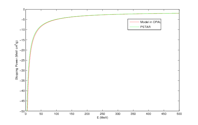
The energy loss in the low-energy region is calculated using semi-empirical fitting formulas of Andersen and Ziegler [65].
where the energy loss is in MeV cm^2/g and \(\epsilon\) is a fitted function of the stopping cross section.
In case of incident protons in the material for energies from 10 keV to 600 keV, the fitting functions are given by:
where \(T_s\) is the kinetic energy (in keV) divided by the proton mass (in amu). For \(T_s\) between 1 and 10 keV, the fitted function is given by:
In case of incident alpha particles for energies from 1 keV to 10 MeV, the stopping power functions is expressed as:
where \(T\) is the kinetic energy in MeV. The numerical values of coefficients of the empirical formulas are showed in Table 44.
The particles lost due to excessive energy loss (final energy null
or lower than LOWENERGYTHR) are recorded in a HDF5 file
(or ASCII if ASCIIDUMP is true).
The loss file name is compound by the associated element name
and the PARTICLEMATTERINTERACTION name.
Energy straggling: For relatively thick absorbers such that the number of collisions is large, the energy loss distribution is shown to be Gaussian in form. For non-relativistic heavy particles the spread \(\sigma_0\) of the Gaussian distribution is calculated by:
where \(\rho\) is the density, \(\Delta s\) is the thickness.
20.2. The Coulomb Scattering
The Coulomb scattering is treated as two independent events: the
multiple Coulomb scattering and the large angle Rutherford scattering.
Using the distribution given in Classical Electrodynamics, by J. D.
Jackson, the multiple- and single-scattering distributions can be
written:
where \(\alpha=\frac{\theta}{<\Theta^2>^{1/2}}=\frac{\theta}{\sqrt 2 \theta_0}\).
The transition point is \(\theta=2.5 \sqrt 2 \theta_0\approx3.5 \theta_0\),
where \(p\) is the momentum, \(\Delta s\) is the step size, and \(X_0\) is the radiation length.
20.2.1. Multiple Coulomb Scattering
Generate two independent Gaussian random variables with mean zero and variance one: \(z_1\) and \(z_2\). If \(z_2 \theta_0>3.5 \theta_0\), start over. Otherwise,
Generate two independent Gaussian random variables with mean zero and variance one: \(z_3\) and \(z_4\). If \(z_4 \theta_0>3.5 \theta_0\), start over. Otherwise,
20.2.2. Large Angle Rutherford Scattering
Generate a random number \(\xi_1\), if \(\xi_1 < \frac{\int_{2.5}^\infty P_S(\alpha)d\alpha}{\int_{0}^{2.5} P_M(\alpha)\;\mathrm{d}\alpha+\int_{2.5}^\infty P_S(\alpha)\;\mathrm{d}\alpha}=0.0047\), sampling the large angle Rutherford scattering.
The cumulative distribution function of the large angle Rutherford scattering is
where \(\xi\) is a random variable. So
Generate a random variable \(P_3\),
if \(P_3>0.5\)
else
The angle distribution after Coulomb scattering is shown in Figure 33. The line is from Jackson’s formula, and the points are simulations with Matlab. For a thickness of \(\Delta s=1e-4\) \(m\), \(\theta=0.5349 \alpha\) (in degree).
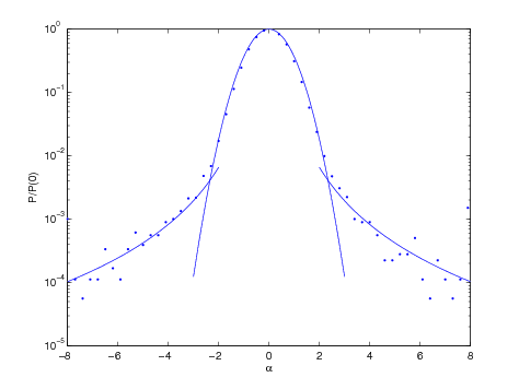
20.3. Beam Stripping physics
Beam stripping physics takes into account two different physical processes: interaction with residual gas and electromagnetic stripping (also called Lorentz stripping). Given the stochastic nature of such interactions, the processes are modeled as a Monte Carlo method.
Both processes are described in the same way: Assuming that particles are normally incident on a homogeneous medium and that they are subjected to a process with a mean free path \(\lambda\) between interactions, the probability of suffering an interaction before reaching a path length \(x\) is:
where \(P(x)\) is the statistic cumulative interaction probability of the process.
20.3.1. Residual gas interaction
The mean free path of the interaction is related with the density of interaction centers and the cross section: \(\lambda=1/N\sigma\). Assuming a beam flux incident in an ideal gas with density \(N\) (number of gas molecules per unit volume under the vacuum condition), the number of particles interacting depends on the gas composition and the different reactions to be considered. Thus, in agreement with Dalton’s law of partial pressures:
where the first summation is over all gas components and the second summation is over all processes for each component.
The fraction loss of the beam for unit of travelled length is: \(f_g=1-e^{-\delta _s /\lambda_{total}}\). For a individual particle, \(f_g\) represents the interaction probability and it is evaluated through an independent random variable each step \(\delta _s\).
Gas stripping could be applied for four different types of incoming
particles: negative hydrogen ions (HMINUS), protons
(PROTON), neutral hydrogen atoms (HYDROGEN) and hydrogen
molecule ions (H2P). Single / Double - electron detachment
or capture reactions are considered for each of them.
Cross sections are calculated according to energy of the particle employing analytic expressions fitted to cross section experimental data. There are three different fitting expressions:
-
Nakai function [59]
where \(\sigma_0\) is a convenient cross section unit (\(\sigma_0 = 1\cdot 10^{-16}\,\text{cm}^2\)), \(E_0\) is the incident projectile energy in keV, \(E_{th}\) is the threshold energy of reaction in keV, and the symbols \(a_i\) denote adjustable parameters.
where \(T_i\) are the Chebyshev orthogonal polynomials.
20.3.2. Electromagnetic stripping
In case of \(H^-\), the second electron is slightly bounded, so
it is relevant to consider the detachement by the magnetic field. The
orthogonal component of the magnetic field to the median plane (read
from Cyclotron element), produces an electric field according to
Lorentz transformation, \(E\!=\!\gamma\beta cB\). The fraction
of particles dissociated by the electromagnetic field during a time
step \(\delta _t\) is:
where \(\tau\) is the particle lifetime in the rest frame, determined theoretically [62]:
where \(z_T\!=\!-\varepsilon_0/eE\) is the outer classical turning radius, \(\varepsilon_0\) is the binding energy, \(p\) is a polarization factor of the ionic wave function, \(k_0^2\!=\!2m(-\varepsilon_0)/\hslash^2\), \(S_{\!0}\) is a spectroscopy coefficient, and the normalization constant is \(N=(2k_0(k_0+\alpha)(2k_0+\alpha))^{1/2} / \alpha\), where \(\alpha\) is a parameter for the ionic potential function.
20.4. The Flow Diagram of ScatteringPhysics Class in OPAL
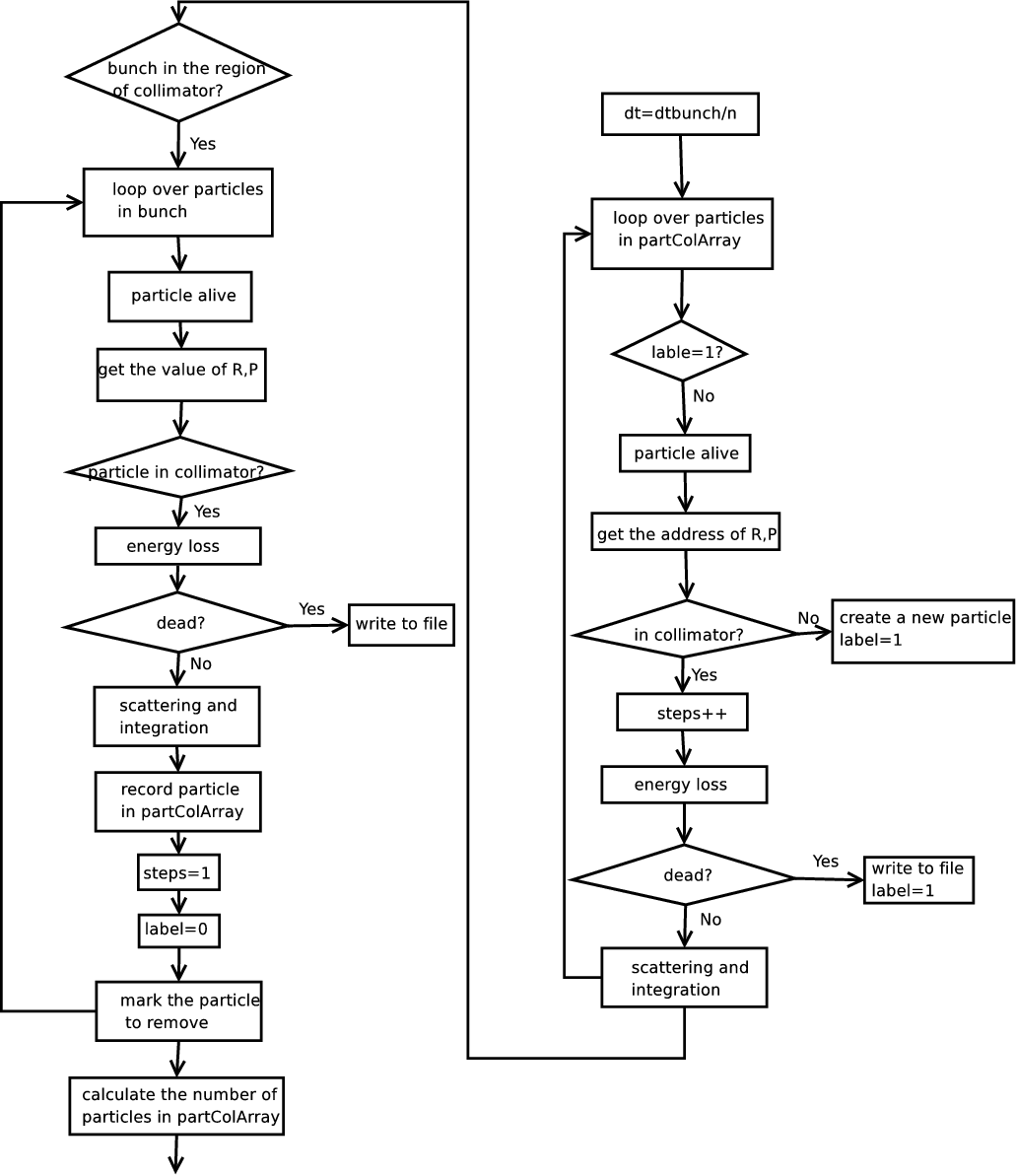
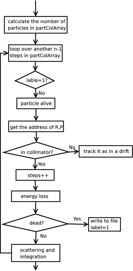
20.4.1. The Substeps
Small step is needed in the routine of ScatteringPhysics.
If a large step is given in the main input file, in the file ScatteringPhysics.cpp, it is divided by a integer number \(n\) to make the step size using for the calculation of scattering physics less than 1.01e-12 s. As shown by Figure 34 and Figure 35 in the previous section, first we track one step for the particles already in the element and the newcomers, then another (n-1) steps to make sure the particles in the element experience the same time as the ones in the main bunch.
Now, if the particle leave the element during the (n-1) steps, we track it as in a drift and put it back to the main bunch when finishing (n-1) steps.
20.5. Available Materials in OPAL
Different materials have been implemented in OPAL for scattering interactions and energy loss calculation. The materials that are supported are listed in Table 43, including the atomic number, \(Z\), the atomic weight, \(A\), the mass density, \(\rho\), the radiation lenght, \(X0\), and the mean excitation energy, \(I\). In addition, the coefficients of the Andersen-Ziegler empirical formulas for the stopping power in the low-energy region are illustrated in Table 44.
| Material (OPAL Name) | Z | A | \(\rho\) [\(g/cm^3\)] | X0 [\(g/cm^2\)] | I [\(eV\)] |
|---|---|---|---|---|---|
|
7 |
14 |
1.205E-3 |
36.62 |
85.7 |
|
13 |
26.9815384 |
2.699 |
24.01 |
166.0 |
|
50 |
101.9600768 |
3.97 |
27.94 |
145.2 |
|
4 |
9.0121831 |
1.848 |
65.19 |
63.7 |
|
26 |
55.251 |
2.52 |
50.13 |
84.7 |
|
29 |
63.546 |
8.96 |
12.86 |
322.0 |
|
79 |
196.966570 |
19.32 |
6.46 |
790.0 |
|
6 |
12.0172 |
2.210 |
42.7 |
78.0 |
|
6 |
12.0172 |
1.88 |
42.7 |
78.0 |
|
6 |
12 |
1.420 |
40.58 |
79.6 |
|
42 |
95.95 |
10.22 |
9.80 |
424.0 |
|
6.702 |
12.88 |
1.400 |
39.95 |
78.7 |
|
22 |
47.867 |
4.540 |
16.16 |
233.0 |
|
10 |
18.0152 |
1 |
36.08 |
75.0 |
| Material (OPAL Name) | A1 | A2 | A3 | A4 | A5 | B1 | B2 | B3 | B4 | B5 |
|---|---|---|---|---|---|---|---|---|---|---|
|
2.954 |
3.350 |
1.683e3 |
1.900e3 |
2.513e-2 |
1.9259 |
0.5550 |
27.15125 |
26.0665 |
6.2768 |
|
4.154 |
4.739 |
2.766e3 |
1.645e2 |
2.023e-2 |
2.5 |
0.625 |
45.7 |
0.1 |
4.359 |
|
1.187e1 |
1.343e1 |
1.069e4 |
7.723e2 |
2.153e-2 |
5.4 |
0.53 |
103.1 |
3.931 |
7.767 |
|
2.248 |
2.590 |
9.660e2 |
1.538e2 |
3.475e-2 |
2.1895 |
0.47183 |
7.2362 |
134.30 |
197.96 |
|
3.519 |
3.963 |
6065.0 |
1243.0 |
7.782e-3 |
5.013 |
0.4707 |
85.8 |
16.55 |
3.211 |
|
3.969 |
4.194 |
4.649e3 |
8.113e1 |
2.242e-2 |
3.114 |
0.5236 |
76.67 |
7.62 |
6.385 |
|
4.844 |
5.458 |
7.852e3 |
9.758e2 |
2.077e-2 |
3.223 |
0.5883 |
232.7 |
2.954 |
1.05 |
|
0.0 |
2.601 |
1.701e3 |
1.279e3 |
1.638e-2 |
3.80133 |
0.41590 |
12.9966 |
117.83 |
242.28 |
|
0.0 |
2.601 |
1.701e3 |
1.279e3 |
1.638e-2 |
3.80133 |
0.41590 |
12.9966 |
117.83 |
242.28 |
|
0.0 |
2.601 |
1.701e3 |
1.279e3 |
1.638e-2 |
3.83523 |
0.42993 |
12.6125 |
227.41 |
188.97 |
|
6.424 |
7.248 |
9.545e3 |
4.802e2 |
5.376e-3 |
9.276 |
0.418 |
157.1 |
8.038 |
1.29 |
|
2.954 |
3.350 |
1683 |
1900 |
2.513e-02 |
1.9259 |
0.5550 |
27.15125 |
26.0665 |
6.2768 |
|
4.858 |
5.489 |
5.260e3 |
6.511e2 |
8.930e-3 |
4.71 |
0.5087 |
65.28 |
8.806 |
5.948 |
|
4.015 |
4.542 |
3.955e3 |
4.847e2 |
7.904e-3 |
2.9590 |
0.53255 |
34.247 |
60.655 |
15.153 |
20.6. Example of an Input File
FX5 is a slit in x direction, the APERTURE is POSITIVE, the first
value in APERTURE is the left part, the second value is the right
part. FX16 is a slit in y direction, the APERTURE is NEGATIVE, the
first value in APERTURE is the down part, the second value is the up
part.
20.7. A Simple Test
A cold Gaussian beam with \(\sigma_x=\sigma_y=5\) mm. The position of the collimator is from 0.01 m to 0.1 m, the half aperture in y direction is \(3\) mm. Figure 36 shows the trajectory of particles which are either absorbed or deflected by a copper slit. As a benchmark of the collimator model in OPAL, Figure 37 shows the energy spectrum and angle deviation at z=0.1 m after an elliptic collimator.
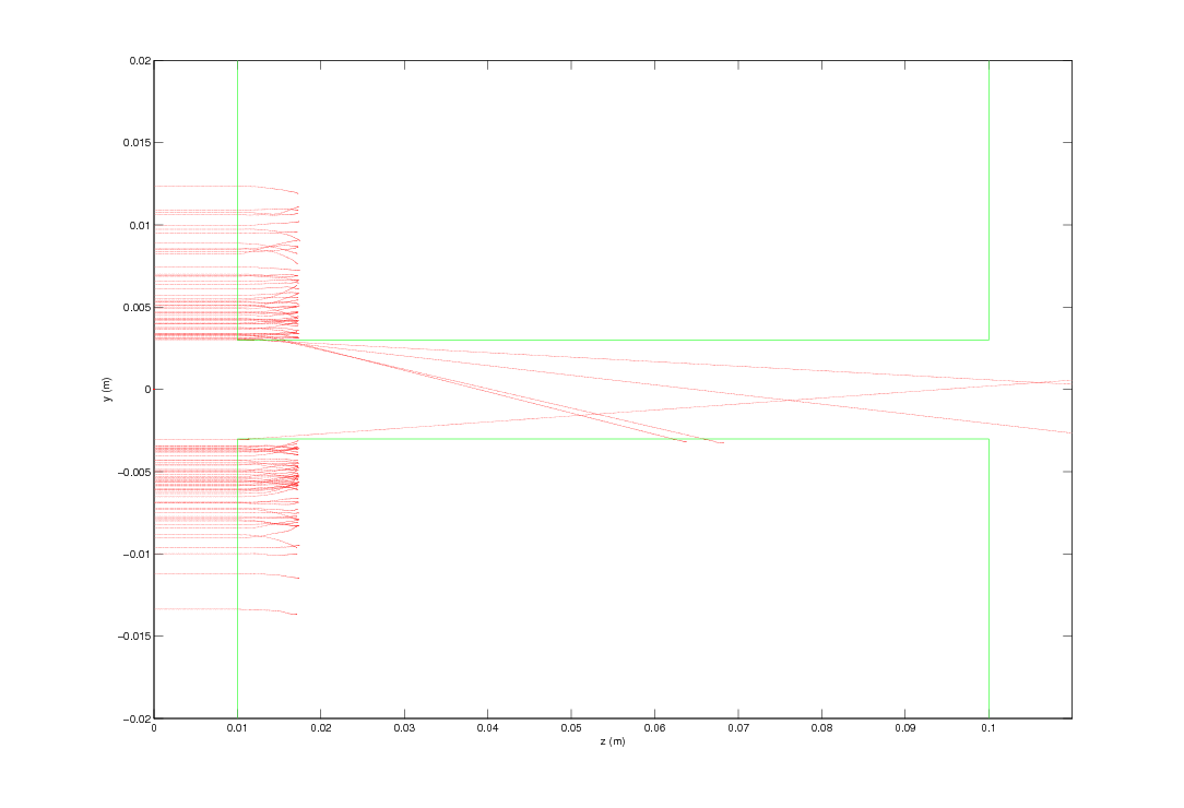
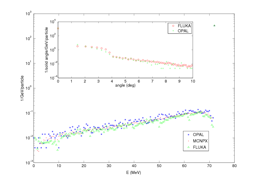
20.8. References
[59] Y. Nakai et al., Cross sections for charge transfer of hydrogen atoms and ions colliding with gaseous atoms and molecules, At. Dat. Nucl. Dat. Tabl., 37, 69 (1987).
[60] T. Tabata and T. Shirai, Analytic Cross Section for Collisions of H+, H2+, H3+, H, H2, and H- with Hydrogen Molecules, At. Dat. Nucl. Dat. Tabl., 76, 1 (2000).
[61] C. F. Barnett, Atomic Data for Fusion Vol. I: Collisions of H, H2, He and Li atoms and ions atoms and molecules, Tech. Rep. ORNL-6086/V1, Oak Ridge National Laboratory (1990).
[62] L. R. Scherk, An improved value for the electron affinity of the negative hydrogen ion, Can. J. Phys., 57, 558 (1979).
[63] Atomic Weights of the Elements 2019, International Union of Pure and Applied Chemistry (IUPAC).
[64] Particle Data Group (PDG), Atomic and Nuclear Properties of Materials for more than 350 materials.
[65] Stopping Powers and Ranges for Protons and Alpha Particles, Tech. Rep. ICRU-49, International Commission on Radiation Units and Measurements (1993)
21. Multi Objective Optimization
Optimization methods deal with finding a feasible set of solutions corresponding to extreme values of some specific criteria. Problems consisting of more than one criterion are called multi-objective optimization problems. Multiple objectives arise naturally in many real world optimization problems, such as portfolio optimization, design, planning and many more [pgnl:06,zepv:00,gala:98,yrss:09,basi:05]. It is important to stress that multi-objective problems are in general harder and more expensive to solve than single-objective optimization problems.
In this chapter we introduce multi-objective optimization problems and discuss techniques for their solution with an emphasis on evolutionary algorithms.
|
Note
|
For multi-objective optimization OPAL uses
opt-pilot developed by Y. Ineichen. opt-pilot
has been fully integrated into OPAL. Instructions can be found on the
opt-pilot wiki page.
|
21.1. Definition
As with single-objective optimization problems, multi-object optimization problems consist of a solution vector and optionally a number of equality and inequality constraints. Formally, a general multi-objective optimization problem has the form
The \(M\) objectives are minimized, subject to \(J\) inequality constraints. An \(n\)-vector contains all the design variables with appropriate lower and upper bounds, constraining the design space.
In contrast to single-objective optimization the objective functions span a multi-dimensional space in addition to the design variable space – for each point in design space there exists a point in objective space. The mapping from the \(n\) dimensional design space to the \(M\) dimensional objective space visualized in Figure 38 is often non-linear. This impedes the search for optimal solutions and increases the computational cost as a result of expensive objective function evaluation. Additionally, depending in which of the two spaces the algorithm uses to determine the next step, it can be difficult to assure an even sampling of both spaces simultaneously.
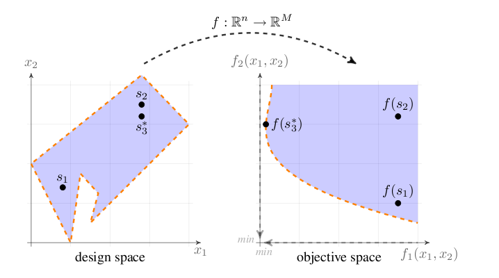
A special subset of multi-objective optimization problems where all objectives and constraints are linear, called Multi-objective linear programs, exhibit formidable theoretical properties that facilitate convergence proofs. In this thesis we strive to address arbitrary multi-objective optimization problems with non-linear constraints and objectives. No general convergence proofs are readily available for these cases.
21.2. Pareto Optimality
In most multi-objective optimization problems we have to deal with conflicting objectives. Two objectives are conflicting if they possess different minima. If all the mimima of all objectives coincide the multi-objective optimization problem has only one solution. To facilitate comparing solutions we define a partial ordering relation on candidate solutions based on the concept of dominance. A solution is said to dominate another solution if it is no worse than the other solution in all objectives and if it is strictly better in at least one objective. A more formal description of the dominance relation is given in [deb:09].
The properties of the dominance relation include transitivity
and asymmetricity, which is necessary for an unambiguous order relation
Using the concept of dominance, the sought-after set of Pareto optimal solution points can be approximated iteratively as the set of non-dominated solutions.
The problem of deciding if a point truly belongs to the Pareto set is NP-hard. As shown in Figure 39 there exist "weaker" formulations of Pareto optimality. Of special interest is the result shown in [paya:01], where the authors present a polynomial (in the input size of the problem and \(1/\varepsilon\)) algorithm for finding an approximation, with accuracy \(\varepsilon\), of the Pareto set for database queries.
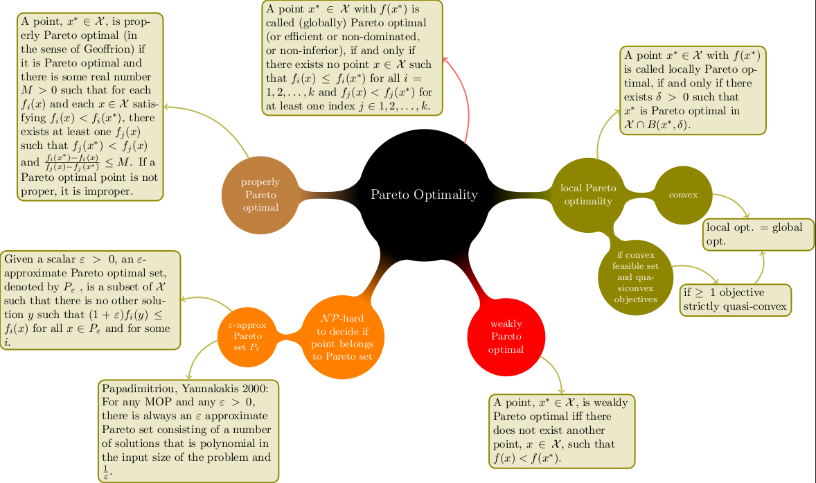
21.3. MOGA Theory
Some links to "What is the tradeoff between population size and the number of generations in genetic algorithms":
21.4. OPAL Commands
21.4.1. Basic Syntax
One needs to define the design variables, objectives and constraints one by one:
d1: DVAR, VARIABLE="x1", LOWERBOUND=-1.0, UPPERBOUND=1.0;
d2: DVAR, VARIABLE="x2", LOWERBOUND=-1.0, UPPERBOUND=1.0;
d3: DVAR, VARIABLE="x3", LOWERBOUND=-1.0, UPPERBOUND=1.0;
This defines three design variables named d1, d2 and d3.
For every variable name e.g. x1 a corresponding variable with underscores _x1_ has to exist in the template input file,
see also the example input file.
Bounds for design variables should always be given.
obj1: OBJECTIVE, EXPR="-statVariableAt('energy', 1.0)";
obj2: OBJECTIVE, EXPR="statVariableAt('emit_x', 1.0)";
This defines two objectives named obj1 and obj2 maximizing the energy and minimizing the emittance in x-direction. The function statVariableAt accecpts as first argument the name of a variable form the .stat output file. As second argument it accepts the location where the variable should be evaluated in s-coordinates.
The optimiser knows several mathematical functions and methods to access output files (see below).
Note that objectives are always minimised, so in this case a solution where the final energy is maximal and the final horizontal emittance is minimal is looked for.
con1: CONSTRAINT, EXPR="statVariableAt('rms_x', 1.0) < 1.0";
con2: CONSTRAINT, EXPR="statVariableAt('numParticles', 1.0) > 1000";
This defines two constraints. The syntax is similar to the OBJECTIVE syntax.
The first constraint consists of only design variables and will be evaluated before the simulation. The second constraint will be evaluated after the simulation.
21.4.2. OPTIMIZE Command
The OPTIMIZE command initiates optimization.
| Attribute | Description |
|---|---|
INPUT |
Path to input file. |
OUTPUT |
Name used in output file generation. |
OUTDIR |
Name of directory used to store generation output files. |
OBJECTIVES |
List of objectives to be used. |
DVARS |
List of optimization variables to be used. |
CONSTRAINTS |
List of constraints to be used. |
INITIALPOPULATION |
Size of the initial population. |
STARTPOPULATION |
A generation file (JSON format) to be started from (optional). In case the number of individuals of the provided file is lower than INITIALPOPULATION, it creates the remaining individuals randomly within the bounds of the DVARS. In case the number of individuals is greater it takes the first INITIALPOPULATION individuals. |
NUM_MASTERS |
Number of master nodes. |
NUM_COWORKERS |
Number processors per worker. |
DUMP_DAT |
Dump old generation data format with frequency, default: false. |
DUMP_FREQ |
Dump generation data format with frequency, default: 1 |
DUMP_OFFSPRING |
Dump offspring (instead of parent population), default: true. |
NUM_IND_GEN |
Number of individuals in a generation. |
MAXGENERATIONS |
Number of generations to run. |
EPSILON |
Tolerance of hypervolume criteria, default: 0.001. |
EXPECTED_HYPERVOL |
The reference hypervolume, default: 0. |
HYPERVOLREFERENCE |
The reference point (real array) for the hypervolume, default: origin. |
CONV_HVOL_PROG |
Converge if change in hypervolume is smaller, default: 0. |
ONE_PILOT_CONVERGE |
default: false |
SOL_SYNCH |
Solution exchange frequency, default: 0. |
INITIAL_OPTIMIZATION |
Optimize speed of first generation creation (useful when number of infeasible solutions large), default: false |
BIRTH_CONTROL |
Enforce strict population sizes, default: false.
If true, population sizes and generations are strictly as defined by |
MUTATION_PROBABILITY |
Mutation probability of individual, default: 0.5. |
MUTATION |
Mutation type of an individual ("OneBit" (single gene), "IndependentBit" (default, multiple genes)) |
GENE_MUTATION_PROBABILITY |
Mutation probability of single gene (used in "IndependentBit" mutation only), default: 0.5. |
RECOMBINATION_PROBABILITY |
Probability for individuals to combine (crossover), default: 0.5. |
CROSSOVER |
Method of child generation based on two individuals ("Blend" (default), "NaiveOnePoint", "NaiveUniform" or "SimulatedBinary") |
SIMBIN_CROSSOVER_NU |
Simulated binary crossover parameter \(\nu\), default: 2.0 |
SIMTMPDIR |
Directory where simulations are run. |
TEMPLATEDIR |
Directory where templates are stored. |
FIELDMAPDIR |
Directory where field maps are stored. |
DISTDIR |
Directory where distributions are stored (optional). |
RESTART_FILE |
H5 file to restart the OPAL simulations from (optional). Each individual copies the H5 to its simulation directory in order to avoid overwriting of the original file. This attributes is used together with RESTART_STEP. |
RESTART_STEP |
Restart from given H5 step (optional). Used together with RESTART_FILE. |
21.4.3. DVAR Command
The DVAR command defines a variable for optimization.
| Attribute | Description |
|---|---|
VARIABLE |
Variable name that should be varied during optimization. |
LOWERBOUND |
Lower limit of the range of values that the variable should assume. |
UPPERBOUND |
Upper limit of the range of values that the variable should assume. |
21.4.4. OBJECTIVE Command
The OBJECTIVE command defines an objective for optimization.
| Attribute | Description |
|---|---|
EXPR |
Expression to minimize during optimization. |
21.4.5. CONSTRAINT Command
The CONSTRAINT command defines a constraint for optimization.
| Attribute | Description |
|---|---|
EXPR |
Expression that should be fulfilled during optimization. |
21.4.6. Available Expressions
The following expressions are available:
The EXPR The optimiser parser knows the following mathematical functions (which are mapped directly to the STL <cmath> functions with the same name):
-
sqrt(x): square root of x -
pow(x,k): x to the power k -
exp(x): e to the power x -
log(x): natural logarithm of x -
ceil(x): round x upward to the smallest integral value that is not less than x -
floor(x): round x downward to smallest integral value that is not greater than x -
fabs(x): absolute value of x -
fmod(x,y): floating point remainder of x/y -
sin(x): sine of angle x (in radians) -
asin(x): the arcsin of x (return value in radians) -
cos(x): cosine of angle x (in radians) -
acos(x): the arc cosine of x (return value in radians) -
tan(x): tangent of angle x (in radians) -
atan(x): the arc tangent of x (return value in radians)
In addition the optimiser parser has one non-STL function:
-
sq(x): square of x
There are several methods to access output data:
| Function | Description |
|---|---|
fromFile(<file>) |
Simple functor that reads vector data from a file. If the file contains more than one value the sum is returned. |
sddsVariableAt(<var>, <refpos>, <sdds_file>) sddsVariableAt(<var>, <refvar>, <refpos>, <sdds_file>) |
A simple expression to get SDDS value near a specific position <refpos> of <refvar> (default: spos) for a variable <var>. If another <refvar> is provided, the values should be monotonically increasing. |
statVariableAt(<var>, <refpos>) statVariableAt(<var>, <refvar>, <refpos>) |
The same as |
sumErrSq(<meas_file>, <var_name>, <sdds_file>) |
A simple expression computing the sum of all measurement errors (given as first and third argument) for a variable (second argument) according to \(result = \frac{1}{n} * \sqrt{\sum_{i=0}^n (measurement_i - value_i)^2}\) |
radialPeak(<file>, <turn>) |
A simple expression to get the n-th peak of a radial probe file.. |
sumErrSqRadialPeak(<meas_file>, <sim_file>, <begin>, <end>) |
A simple expression computing the sum of all peak errors (given as first and second argument) for a range of peaks (third argument and fourth argument) \(result = \frac{1}{n} * \sqrt{\sum_{i=start}^{end} (measurement_i - value_i)^2}\) |
probVariableWithID(<var>, <id>, <probe_file>) |
Returns the value of the variable (first argument) with a certain ID (second argument) from probe loss file (third argument). |
septum(<probe>) |
Returns the minimum bin count between the last and second last turn at the given probe. It uses the <probe>.hist and <probe>.peaks file (cf. probe element). |
21.4.7. Example Input File
05-DL_QN3.in for the optimization using the template file tmpl/05-DL_QN3.tmpl:OPTION, ECHO=FALSE;
OPTION, INFO=TRUE;
TITLE, STRING="OPAL Test MAB, 2016-10-13";
REAL up = 0.0000977;
REAL loc = 2.0;
dv0: DVAR, VARIABLE="QDX1_K1", LOWERBOUND=0, UPPERBOUND=35;
dv1: DVAR, VARIABLE="QDX2_K1", LOWERBOUND=0, UPPERBOUND=34;
dv2: DVAR, VARIABLE="QFX1_K1", LOWERBOUND=-35, UPPERBOUND=0;
drmsx: OBJECTIVE, EXPR="fabs(statVariableAt('rms_x', ${loc}) - ${up})";
drmsy: OBJECTIVE, EXPR="fabs(statVariableAt('rms_y', ${loc}) - 0.0001833)";
goalfun: OBJECTIVE, EXPR="statVariableAt('rms_x', 2.00)";
OPTIMIZE, INPUT="tmpl/05-DL_QN3.tmpl", OBJECTIVES = {drmsx, drmsy, goalfun},
DVARS = {dv0, dv1, dv2}, INITIALPOPULATION=5, MAXGENERATIONS=3,
NUM_IND_GEN=3, MUTATION_PROBABILITY=0.43,
NUM_MASTERS=1, NUM_COWORKERS=1, SIMTMPDIR="simtmpdir",
TEMPLATEDIR="tmpl", FIELDMAPDIR="fieldmaps", OUTPUT="optLinac",
OUTDIR="results";
QUIT;
tmpl/05-DL_QN3.tmpl.Note that the design variables start and end with underscores:
OPTION, ECHO=FALSE;
OPTION, INFO=FALSE;
OPTION, PSDUMPFREQ=1000000;
OPTION, STATDUMPFREQ=20;
OPTION, CZERO=TRUE;
OPTION, IDEALIZED=TRUE;
OPTION, VERSION=10900;

TITLE, STRING="OPAL Test MAB, 2016-10-13";

//////////////////////////////
// Begin Content
//////////////////////////////

REAL SOL  = 2.9979246E8;
REAL Pcen = 100.0E6;
REAL BRho = Pcen/SOL;
REAL QK1  = 6.2519;
REAL QSTR = QK1*BRho/2.0;

QDX1: QUADRUPOLE, ELEMEDGE=0.0,  L=0.10, APERTURE="circle(0.1)",
                 K1=_QDX1_K1_ * BRho / 2;
QFX1: QUADRUPOLE, ELEMEDGE=0.91, L=0.20, APERTURE="circle(0.1)",
                 K1=_QFX1_K1_ * BRho / 2;
QDX2: QUADRUPOLE, ELEMEDGE=1.92, L=0.10, APERTURE="circle(0.1)",
                 K1=_QDX2_K1_ * BRho / 2;

FODO: LINE = (QDX1, QFX1, QDX2);

//////////////////////////////
// Begin Summary
//////////////////////////////

FODO_Full: LINE = (FODO), ORIGIN={0,0,0}, ORIENTATION={0.0, 0.0, 0.0};

//////////////////////////////
// End Summary
//////////////////////////////

// SC calculations on:
Fs1:FIELDSOLVER, FSTYPE = FFT, MX = 16, MY = 16, MT = 16,
                  PARFFTX = true, PARFFTY = true, PARFFTT = true,
                  BCFFTX = open, BCFFTY = open, BCFFTT = open,
                  BBOXINCR = 1, GREENSF = INTEGRATED;
Fs2:FIELDSOLVER, FSTYPE = NONE, MX = 16, MY = 16, MT = 16,
                 PARFFTX = true, PARFFTY = true, PARFFTT = true,
                 BCFFTX = open, BCFFTY = open, BCFFTT = open,
                 BBOXINCR = 1, GREENSF = INTEGRATED;


Dist2: DISTRIBUTION, TYPE="FROMFILE", FNAME="fodo_opal.in";


REAL MINSTEPFORREBIN = 500;

REAL qb=77.0e-12;
REAL bfreq=1300.0E6;
REAL bcurrent=qb*bfreq;

beam1: BEAM, PARTICLE = ELECTRON, pc = P0, NPART = 5000, BFREQ = bfreq,
             BCURRENT = bcurrent, CHARGE = -1;

SELECT, LINE=FODO_Full;

TRACK, LINE=FODO_Full, BEAM=beam1, MAXSTEPS={6e5}, DT={1e-12}, ZSTOP={2.02};

RUN, METHOD = "PARALLEL-T", BEAM = beam1, FIELDSOLVER = Fs2, DISTRIBUTION = Dist2;

ENDTRACK;

QUIT;
Run OPAL with:
mpirun /path/to/opal --info 5 05-DL_QN3.in21.4.8. Output
The solutions for each generation will be saved in either a plain ASCII (if DUMP_DAT true) and JSON format.
The Pareto front of all individuals is in a JSON file, ParetoFront_.json.
There are three log files opt.trace.0, opt-progress.0 and pilot.trace.0 that log the job management.
E.g. to count the total number of dispatched simulations:
cat opt.trace.0 | grep dispatched | wc -lor to count all invalid simulations:
cat opt.trace.0 | grep invalid | wc -l22. Sampler
This is a modification of the optimiser. Instead of performing a multi-objective optimisation, it creates samples of the design variables and runs those simulations. This feature can be used for example as training / validation of neural networks or uncertainty quantification (UQ).
22.1. OPAL Commands
It uses almost the same syntax as the optimiser.
22.1.1. Basic Syntax
One needs to define the design variables and their sampling method. The syntax for design variables is described in the section DVAR Command.
22.1.2. SAMPLE Command
It allows random (RASTER=false) and raster mode.
| Attribute | Description |
|---|---|
RASTER |
Boolean to choose how the sample spaces for the DVARS are combined, see below, (default: true) |
INPUT |
Path to input file. |
OUTPUT |
Name used for the output of the result. |
OUTDIR |
Name of directory where the simulations are run and the result file is stored. |
DVARS |
List of design variables to be used. |
OBJECTIVES |
List of objectives which are evaluated for each simulation. The results are stored to the result file |
SAMPLINGS |
List of sample methods to be used. |
NUM_MASTERS |
Number of master nodes. |
NUM_COWORKERS |
Number processors per worker. |
TEMPLATEDIR |
Directory where templates are stored. |
FIELDMAPDIR |
Directory where field maps are stored. |
DISTDIR |
Directory where distributions are stored (optional). |
KEEP |
List of file extensions (e.g. STAT, H5) that shouldn’t be deleted. If nothing is specified, all files are kept. If objectives are defined and list is empty all files are deleted. |
RESTART_FILE |
H5 file to restart the OPAL simulations from (optional). Each individual copies the H5 to its simulation directory in order to avoid overwriting of the original file. This attributes is used together with RESTART_STEP. |
RESTART_STEP |
Restart from given H5 step (optional). Used together with RESTART_FILE. |
JSON_DUMP_FREQ |
Defines how often new individuals are appended to the final JSON file i.e. every time JSON_DUMP_FREQ samples finished they are written. (default: All individuals are written at the end) |
The difference between RASTER = TRUE and RASTER = FALSE can be depicted in the following figure.
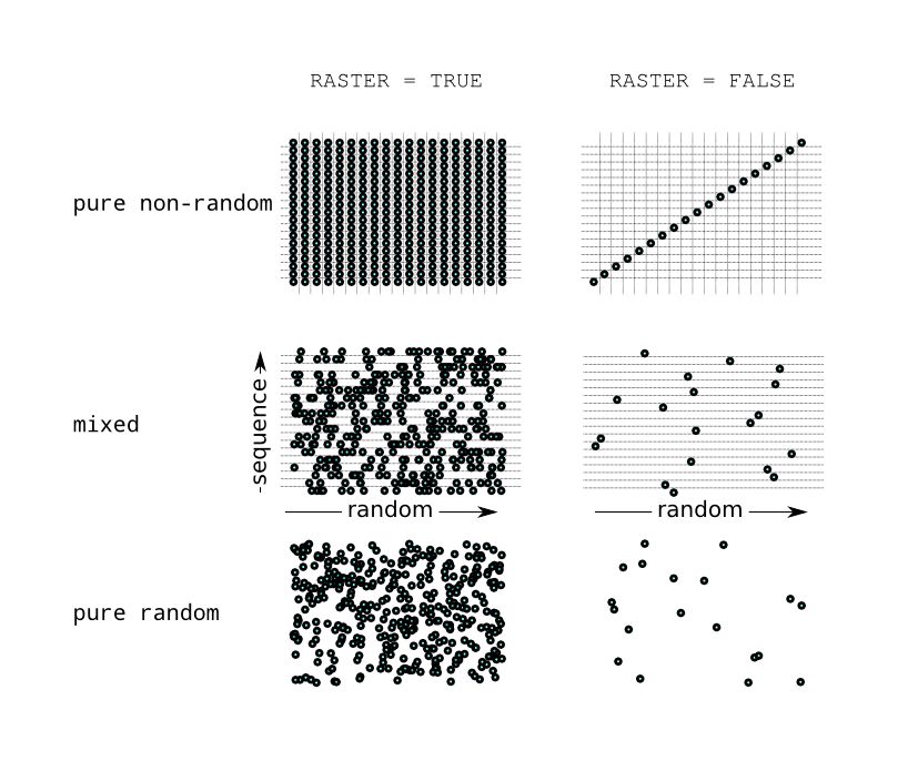
The two sampling methods differ in the number of samples since with RASTER = TRUE every combination of individual sampling is computed. Thus the total number is \(N = N_1 \times N_2 \times \ldots \times N_n\) where \(n\) is the number of DVARS. If for some DVAR a random sampling is chosen then for every sampling point a new random number is computed. With RASTER = FALSE the number of sampling points is \(N = \min(N_1, N_2,\ldots, N_n)\), each item of a sequence is used only once.
22.1.3. SAMPLING Command
| Attribute | Description |
|---|---|
VARIABLE |
Name of the design variable. |
TYPE |
Sampling method (see next section). |
RANDOM |
Boolean to control whether sampling mode is random or sequential. Default is sequential. |
SEED |
Seed for random sampling (default: 42). |
STEP |
Increment for randomized sequences (default: 1) |
FNAME |
File to read the samples from. |
N |
Number of samples per this design variable. In case of random mode, the minimum value over all design variables is used. |
22.1.4. Available Sampling Methods
| Method | Description |
|---|---|
FROMFILE |
The samples are provided by a file. A column represents the values of a design variable. The first line is the header reading the variable name. Not all variables need to be provided in the file. This allows also reading variables from different files. |
UNIFORM |
In sequence mode: Generates an equidistant sequence taking the lower and upper bound of the design variable command as limits. In random mode: Uniform random sampling of floats. It takes the lower and upper bound of the design variable command as limits. |
UNIFORM_INT |
In sequence mode: Generates an equidistant sequence of integers taking the lower and upper bound of the design variable command as limits. In random mode: Uniform random sampling of integers. It takes the lower and upper bound of the design variable command. |
GAUSSIAN |
In sequence mode: Generates a sequence with a gaussian distribution taking the difference between upper and lower bound of the design variable as \(10\;\sigma\). In random mode: Gaussian random sampling of floats. The upper and lower bound are the \(\pm 5\; \sigma\) limits of the distribution. |
LATIN_HYPERCUBE |
In random mode only. Each dimension is discretized into N (i.e. number of samples) equally distant bins. In order to sample a bin in every dimension is randomly selected where the same bin in a dimension occurs only once (exclusive sampling). |
RANDOM_SEQUENCE_UNIFORM_INT |
In random mode only. Similar to UNIFORM_INT in sequence mode but the values are returned randomly and a value may occur several times or never. Together with the STEP attribute. |
RANDOM_SEQUENCE_UNIFORM |
In random mode only. Similar to UNIFORM in sequence mode but the values are returned randomly and a value may occur several times or never. Together with the STEP attribute. |
22.2. Example Input File
OPTION, INFO=TRUE;

// Design variables
nstep:  DVAR, VARIABLE="nstep", LOWERBOUND=10,     UPPERBOUND=40;
MX:     DVAR, VARIABLE="MX",    LOWERBOUND=16,     UPPERBOUND=32;

// Sampling methods
SM1: SAMPLING, VARIABLE="nstep", TYPE="FROMFILE",    FNAME="samples.dat";
SM2: SAMPLING, VARIABLE="MX",    TYPE="UNIFORM_INT", SEED=122, N = 6;

SAMPLE,
    RASTER          = false,
    DVARS           = {nstep, MX},
    SAMPLINGS       = {SM1, SM2},
    INPUT           = "Ring.tmpl",
    OUTPUT          = "RingSample",
    OUTDIR          = "RingSample",
    TEMPLATEDIR     = "template",
    FIELDMAPDIR     = "Fieldmaps",
    NUM_MASTERS     = 1,
    NUM_COWORKERS   = 1;
QUIT;
The samples of nstepsamples.dat
MX    nstep
16    10
17    11
18    12
19    13
20    14
21    15
22    16
23    17
24    18
25    19
Although the file contains samples for MXRing.tmpl
Option, ECHO=FALSE;
Option, PSDUMPFREQ=100000;
Option, SPTDUMPFREQ = 10;
Option, PSDUMPEACHTURN=false;
Option, REPARTFREQ=20;
Option, ECHO=FALSE;
Option, STATDUMPFREQ=1;
Option, CZERO=FALSE;
Option, MEMORYDUMP=TRUE;
Option, TELL=TRUE;
Option, VERSION=10900;

Title,string="OPAL-cycl: the first turn acceleration in PSI 590MeV Ring";

REAL Edes=.072;
REAL gamma=(Edes+PMASS)/PMASS;
REAL beta=sqrt(1-(1/gamma^2));
REAL gambet=gamma*beta;
REAL P0 = gamma*beta*PMASS;
REAL brho = (PMASS*1.0e9*gambet) / CLIGHT;

//value,{gamma,brho,Edes,beta,gambet};

REAL phi01=139.4281;
REAL phi02=phi01+180.0;
REAL phi04=phi01;
REAL phi05=phi01+180.0;
REAL phi03=phi01+10.0;

REAL volt1st=0.9;
REAL volt3rd=0.9*4.0*0.112;

REAL turns = 1;
REAL nstep=_nstep_;

REAL frequency=50.650;
REAL frequency3=3.0*frequency;

ring: Cyclotron, TYPE="RING", CYHARMON=6, PHIINIT=0.0,
	PRINIT=-0.000174, RINIT=2130.0, SYMMETRY=8.0, RFFREQ=frequency,
	FMAPFN="s03av.nar";

rf0: RFCavity, VOLT=volt1st, FMAPFN="Cav1.dat", TYPE="SINGLEGAP",
	FREQ=frequency, RMIN = 1900.0, RMAX = 4500.0, ANGLE=35.0,  PDIS = 416.0,
	GAPWIDTH = 220.0, PHI0=phi01;

rf1: RFCavity, VOLT=volt1st, FMAPFN="Cav1.dat", TYPE="SINGLEGAP",
	FREQ=frequency, RMIN = 1900.0, RMAX = 4500.0, ANGLE=125.0, PDIS = 416.0,
	GAPWIDTH = 220.0, PHI0=phi02;

rf2: RFCavity, VOLT=volt3rd, FMAPFN="Cav3.dat", TYPE="SINGLEGAP",
	FREQ=frequency3,RMIN = 1900.0, RMAX = 4500.0, ANGLE=170.0, PDIS = 452.0,
	GAPWIDTH = 250.0, PHI0=phi03;

rf3: RFCavity, VOLT=volt1st, FMAPFN="Cav1.dat", TYPE="SINGLEGAP",
	FREQ=frequency, RMIN = 1900.0, RMAX = 4500.0, ANGLE=215.0, PDIS = 416.0,
	GAPWIDTH = 220.0, PHI0=phi04;

rf4: RFCavity, VOLT=volt1st, FMAPFN="Cav1.dat", TYPE="SINGLEGAP",
	FREQ=frequency, RMIN = 1900.0, RMAX = 4500.0, ANGLE=305.0, PDIS = 416.0,
	GAPWIDTH = 220.0, PHI0=phi05;

l1:   Line = (ring,rf0,rf1,rf2,rf3,rf4);

Dist1:DISTRIBUTION, TYPE=gauss,
	sigmax = 2.0e-03,
	sigmapx = 1.0e-7,
	corrx = 0.0,
	sigmay = 2.0e-03,
	sigmapy = 1.0e-7,
	corry = 0.0,
	sigmat = 2.0e-03,
	sigmapt = 3.394e-4,
	corrt=0.0;

Fs1:FIELDSOLVER, FSTYPE=FFT, MX=_MX_, MY=16, MT=16,
	PARFFTX=true, PARFFTY=true, PARFFTT=true,
	BCFFTX=open, BCFFTY=open, BCFFTT=open, BBOXINCR=2;

beam1: BEAM, PARTICLE=PROTON, pc=P0, NPART=8192, BCURRENT=1.0E-3, CHARGE=1.0,
             BFREQ= frequency;

Select, Line=l1;

TRACK,LINE=l1, BEAM=beam1, MAXSTEPS=nstep*turns, STEPSPERTURN=360,TIMEINTEGRATOR="RK-4";
 run, method = "CYCLOTRON-T", beam=beam1, fieldsolver=Fs1, distribution=Dist1;
endtrack;

Stop;
Appendix A: OPAL Language Syntax
Words in italic font are syntactic entities, and characters in
monospaced font must be entered as shown. Comments are given in bold
font.
A.1. Statements
comment |
: |
|
| |
|
|
identifier |
: |
|
integer |
: |
|
string |
: |
|
| |
|
|
command |
: |
keyword attribute-list |
| |
label |
|
keyword |
: |
identifier |
label |
: |
identifier |
attribute-list |
: |
empty |
| |
attribute-list |
|
attribute |
: |
attribute-name // only for logical attribute |
| |
attribute-name |
|
// expression evaluated |
||
| |
attribute-name |
|
// expression retained |
||
attribute-name |
: |
identifier |
attribute-value |
: |
string-expression |
| |
logical-expression |
|
| |
real-expression |
|
| |
array-expression |
|
| |
constraint |
|
| |
variable-reference |
|
| |
place |
|
| |
range |
|
| |
token-list |
|
| |
token-list-array |
|
| |
regular-expression |
A.2. Real expressions
real-expression |
: |
real-term |
| |
|
|
| |
|
|
| |
real-expression |
|
| |
real-expression |
|
real-term |
: |
real-factor |
| |
real-term |
|
| |
real-term |
|
real-factor |
: |
real-primary |
| |
real-factor |
|
real-primary |
: |
real-literal |
| |
symbolic-constant |
|
| |
|
|
| |
real-name |
|
| |
array |
|
| |
object-name |
|
| |
object-name |
|
| |
table-reference |
|
| |
real-function |
|
| |
real-function |
|
| |
real-function |
|
| |
function-of-array |
|
| |
|
|
real-function |
: |
|
| |
|
|
| |
|
|
| |
|
|
| |
|
|
| |
|
|
| |
|
|
| |
|
|
| |
|
|
| |
|
|
| |
|
|
| |
|
|
| |
|
|
| |
|
|
| |
|
|
| |
|
|
| |
|
|
| |
|
|
| |
|
|
| |
|
|
| |
|
|
| |
|
|
| |
|
|
function-of-array |
: |
|
| |
|
|
| |
|
|
| |
|
A.3. Real variables and constants:
real-prefix |
: |
empty |
| |
|
|
| |
|
|
| |
|
|
real-definition |
: |
real-prefix real-name |
// expression evaluated |
||
| |
real-prefix real-name |
|
// expression retained |
||
symbolic-constant |
: |
|
| |
|
|
| |
|
|
| |
|
|
| |
|
|
| |
|
|
| |
|
|
| |
|
|
| |
|
|
| |
|
|
| |
|
|
| |
|
|
| |
|
|
| |
|
|
| |
real-name |
|
real-name |
: |
identifier |
object-name |
: |
identifier |
table-name |
: |
identifier |
column-name |
: |
identifier |
A.4. Logical expressions:
logical-expression |
: |
and-expression |
| |
logical-expression || and-expression |
|
and-expression |
: |
relation |
| |
and-expression |
|
relation |
: |
logical-name |
| |
|
|
| |
|
|
| |
real-expression relation-operator real-expression |
|
logical-name |
: |
identifier |
relation-operator |
: |
|
| |
|
|
| |
|
|
| |
|
|
| |
|
|
| |
|
A.5. Logical variables:
logical-prefix |
: |
|
| |
|
|
logical-definition |
: |
logical-prefix logical-name |
// expression evaluated |
||
| |
logical-prefix logical-name `:=` logical-expression |
|
// expression retained |
A.6. String expressions:
string-expression |
: |
string |
| |
identifier // taken as a string |
|
| |
string-expression |
A.7. String constants:
string-prefix |
: |
|
string-definition |
: |
string-prefix string-name |
// expression evaluated |
||
| |
string-prefix string-name |
|
// expression retained |
A.8. Real array expressions:
array-expression |
: |
array-term |
| |
|
|
| |
|
|
| |
array-expression |
|
| |
array-expression |
|
array-term |
: |
array-factor |
| |
array-term |
|
| |
array-term |
|
array-factor |
: |
array-primary |
| |
array-factor |
|
array-primary |
: |
|
| |
array-reference |
|
| |
real-function |
|
| |
|
|
array-literal |
: |
real-expression |
| |
array-literal |
|
array-reference |
: |
array-name |
| |
object-name |
|
array-name |
: |
identifier |
A.9. Real array definitions:
array-prefix |
: |
|
array-definition |
: |
array-prefix array-name |
| |
array-prefix array-name |
A.10. Constraints:
constraint |
: |
array-expression constraint-operator array-expression |
constraint-operator |
: |
|
| |
|
|
| |
|
A.11. Variable references:
variable-reference |
: |
real-name |
| |
object-name |
A.12. Token lists:
token-list |
: |
anything-except-comma |
token-list-array |
: |
token-list |
| |
token-list-array |
A.13. Regular expressions:
regular-expression |
: |
|
Appendix B: OPAL-t Field Maps
B.1. Introduction
In this chapter details of the different types of field maps in OPAL-t are presented. OPAL-t can use many different types of field maps input in several different file formats. What types of maps are supported and in what format has tended to be a function mostly of what developers have needed, and to a lesser extent what users have asked for. The list below shows all field maps that are currently supported and also field maps that are not yet supported, but on the list of things to do when we get a chance.
B.2. Comments in Field Maps
The possibility to add comments (almost) everywhere in field map files is common to all field maps. Comments are initiated by a # and contain the rest of a line. Comments are accepted at the beginning of the file, between the lines and at the end of a line. If in the following sections two values are shown on one line then they have to be on the same line. They should not be separated by a comment and, consequently, be on different lines. Three examples of valid comments:
# This is valid a comment
1DMagnetoStatic 40 # This is another valid comment
-60.0 60.0 9999
  # and this is also a valid comment
0.0 2.0 199
The following examples will break the parsing of the field maps:
1DMagnetoStatic # This is an invalid comment
40
-60.0 60.0 # This is another invalid comment # 9999
0.0 2.0 199
B.3. Normalization
All field maps that are in ASCII are normalized with the maximum
absolute value of the longitudinal field on the axis. The only
exceptions is the type 1DProfile1. This behavior can be disabled by
adding FALSE at the end of the first line of the field map.
B.4. Field Map Warnings and Errors
If OPAL-t encounters an error while parsing a field map it disables the corresponding element, outputs a warning message and continues the simulation. The following messages may be output:
************ W A R N I N G ***********************************
THERE SEEMS TO BE SOMETHING WRONG WITH YOUR FIELD MAP file.t7.
There are only 10003 lines in the file, expecting more.
Please check the section about field maps in the user manual.
**************************************************************
In this example there is something wrong with the number of grid spacings provided in the header of the file. Make sure that you provide the number of grid spacings and not the number of grid points! The two numbers always differ by 1.
************ W A R N I N G ***********************************
THERE SEEMS TO BE SOMETHING WRONG WITH YOUR FIELD MAP file.t7.
There are too many lines in the file, expecting only 10003 lines.
Please check the section about field maps in the user manual.
**************************************************************
Again there seems to be something wrong with the number of grid spacings provided in the header. In this example OPAL-t found more lines than it expected. Note that comments and empty lines at the end of a file are ignored such that they don’t cause this warning.
************ W A R N I N G ***********************************
THERE SEEMS TO BE SOMETHING WRONG WITH YOUR FIELD MAP file.t7.
_error_msg_
expecting: '_expecting_' on line 3,
found instead: '_found_'.
**************************************************************
Where “_error_msg_” is either
|
If OPAL-t expects more values on this line. |
|
If OPAL-t expects less values on this line. |
|
If OPAL-t found e.g. characters instead of an integer number. |
“_expecting_” is replaced by the types of values OPAL-t expects on the
line. E.g. it could be replaced by double double int. Finally
“_found_” is replaced by the actual content of the line without any
comment possibly following the values. If line 3 of a file consists of
-60.0 60.0 # This is an other invalid comment # 9999 OPAL-t will
output -60.0 60.0.
************** W A R N I N G *********************************
DISABLING FIELD MAP file.t7 SINCE FILE COULDN'T BE FOUND!
**************************************************************
This warning could be issued if the file name is mistyped or otherwise if the file couldn’t be read.
************ W A R N I N G **********************************
THERE SEEMS TO BE SOMETHING WRONG WITH YOUR FIELDMAP file.t7.
Could not determine the file type.
Please check the section about field maps in the user manual.
*************************************************************
In this case OPAL-t didn’t recognize the string of characters which identify the type of field map stored in the file.
For one-dimensional field maps an other warning may be issued:
* ************ W A R N I N G ***************************************************
* IT SEEMS THAT YOU USE TOO FEW FOURIER COMPONENTS TO SUFFICIENTLY WELL        *
* RESOLVE THE FIELD MAP 'file.T7'.                                             *
* PLEASE INCREASE THE NUMBER OF FOURIER COMPONENTS!                            *
* The ratio (f_i - F_i)^2 / F_i^2 is 0.019685 and                              *
* the ratio (max_i(|f_i - F_i|) / max_i(|F_i|) is 0.019023.                    *
* Here F_i is the field as in the field map and f_i is the reconstructed       *
* field.                                                                       *
* The lower limit for the two ratios is 1e-2                                   *
* ******************************************************************************
This warning is issued when the low pass filter that is applied to the field sampling uses too few Fourier coefficients. In this case increase the number of Fourier coefficients, see the next section for details. The relevant criteria are that
and
where \(F_{z_i}\) is the field sampling as in the file and \(\tilde{F}_{z,i}\) is the one-dimensional field reconstructed from the result received after applying the low pass filter.
B.5. Types and Format
Field maps in OPAL-t come in three basic types:
-
2D or 3D field map. For this type of map, a field is specified on a grid and linear interpolation is used to find field values at intermediate points.
-
1D on axis field map. For this type of map, one on-axis field profile is specified. OPAL-t calculates a Fourier series from this profile and then uses the first, second and third derivatives of the series to compute the off-axis field values. (This type of field is very smooth numerically, but can be inaccurate far from the field axis.) Only a few (user specified) terms from the Fourier series are used.
-
Enge function [66] field map. This type of field map uses Enge functions to describe the fringe fields of a magnet. Currently, this is only used for
RBENDandSBENDelements see RBend (OPAL-t) and SBend (OPAL-t).
It is important to note that in all cases, the input field map will be normalized so that the peak field magnitude value on axis is equal to either 1 MV/m in the case of electric field maps (static or dynamic), or 1 T in the case of magnetic field maps. (The sign of the values from the field map are preserved.) Therefore, the field multiplier for the map in your simulation will be the peak field value on axis in those respective units.
Depending on the field map type, OPAL-t uses different length units (either cm or meters). This is due to the origin programs of the field maps used (e.g. Poisson/Superfish [67] uses cm). So be careful.
There are no required field extensions for any OPAL-t field map (e.g. .T7, .dat etc.). OPAL-t determines the type of field map by a string descriptor which is the first element on the first line of the file. Below we list the possible descriptors. (Note that we list all of the descriptors/field map types that we plan to eventually implement. Not all of them are, which is indicated in the description.)
- 1DElectroStatic
-
1D electrostatic field map. 1D field maps are described by the on-axis field.
Not implemented yet. A work around is to use a 1DDynamic field map with a very low frequency. - 1DMagnetoStatic
-
1D magnetostatic field map. See 1DMagnetoStatic.
- AstraMagnetoStatic
-
1D magnetostatic field map with possibly non-equidistant sampling. This file type is compatible with ASTRA field maps with small changes. See AstraMagnetostatic.
- 1DDynamic
-
1D dynamic electromagnetic field map. See 1DDynamic.
- AstraDynamic
-
1D dynamic electromagnetic field map with possibly non-equidistant sampling. This file type is compatible with ASTRA field maps with small changes. See AstraDynamic.
- 1DProfile1
-
This type of field map specifies the Enge functions (see [66]) for the entrance and exit fringe fields of a magnet. Currently this type of field map is only used by
RBENDandSBENDelements see RBend (OPAL-t) and SBend (OPAL-t). See 1DProfile1. - 2DElectroStatic
-
2D electrostatic field map. 2D field maps are described by the electromagnetic field in one half-plane. See 2DElectroStatic.
- 2DMagnetoStatic
-
2D magnetostatic field map. Other than this descriptor at the head of the file, the format for this field map type is identical to the T7 file format as produced by Poisson [67]. See 2DMagnetoStatic.
- 2DDynamic
-
2D dynamic electromagnetic field map. Other than this descriptor at the head of the file, the format for this field map type is identical to the T7 field format as produced by Superfish [67]. See 2DDynamic.
- 3DElectroStatic
-
3D electrostatic field map.
Not implemented yet. - 3DMagnetoStatic
-
3D magnetostatic field map, see 3DMagnetoStatic.
- 3DMagnetoStatic_Extended
-
2D magnetostatic field map of field on mid-plane that OPAL extends to 3D.
- 3DDynamic
-
3D dynamic electromagnetic field map. See 3DDynamic.
We will give examples and descriptions of each of the implemented field map types in the sections below.
B.6. Field Map Orientation
In the case of 2D and 3D field maps an additional string has to be provided describing the orientation of the field map.
For 2D field maps this can either be
- XZ
-
if the primary direction is in z direction and the secondary in r direction.
- ZX
-
if the primary direction is in r direction and the secondary in z direction.
For 3D field maps this can be
- XYZ
-
if the primary direction is in z direction, the secondary in y direction and the tertiary in x direction
Each line after the header corresponds to a grid point of the field map. This point can be referred to by two indices in the case of a 2D field map and three indices in the case of a 3D field map, respectively. Each column describes either \(E_z,\; E_r,\; B_z,\; B_r\; \text{or}\;H_{\phi}\) in the 2D case and \(E_x\;, E_y\;, E_z,\; B_x,\; B_y,\;B_z\) in the 3D case.
By primary, secondary and tertiary direction is meant the following (see also Figure 41):
-
The index of the primary direction increases the fastest, the index of the tertiary direction the slowest.
-
The order of the columns is accordingly: if the z direction in an 2D electrostatic field map is the primary direction then \(E_z\) is on the first column, \(E_r\) on the second. For all other cases it’s analogous.
-
For the 2D dynamic case in XZ orientation there are four columns: \(E_z\), \(E_r\), \(|E|\) (unused) and \(H_{\phi}\) in that order. In the other orientations the first and the second columns are interchanged ,but the third and fourth columns are unchanged.
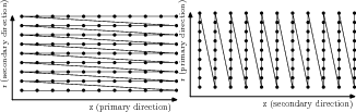
B.7. FAST Attribute for 1D Field Maps
For some 1D field maps, there exists a Boolean attribute, FAST, which
can be used to speed up the calculation. When set to true
(FAST = TRUE), OPAL-t will generate a 2D internal field map and then
use bi-linear interpolation to calculate field values during the
simulation, rather than the generally slower Fourier coefficient
technique. The caution here is that this can introduce unwanted
numerical noise if you set the grid spacing too coarse for the 2D map.
As a general warning: be wise when you choose the type of field map to
be used! Figure 42 shows three pictures of the
longitudinal phase space after three gun simulations using different
types of field maps. In the first picture we
used a 1DDynamic field map see 1DDynamic resulting in a smooth
longitudinal distribution. In the middle picture we set the
FAST attribute to true, resulting in some fine structure in the phase
space due to the bi-linear interpolation of the internally generated 2D
field map. Finally, in the last figure, we
generated directly a 2D field map from Superfish [67]. Here we
could observe two different structures: first the fine structure,
stemming from the bi-linear interpolation, and secondly a much stronger
structure of unknown origin, but presumably due to errors in the
Superfish [67] interpolation algorithm.
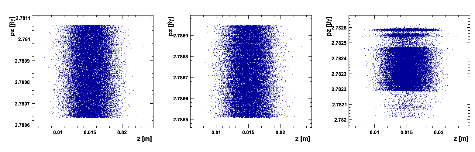
FAST switch, and a 2D field map of the gun generated by Superfish.B.8. 1DMagnetoStatic
1DMagnetoStatic 40
-60.0 60.0 9999
  0.0  2.0 199
  0.00000e+00
  4.36222e-06
  8.83270e-06
  + 9'994 lines
  1.32490e-05
  1.73710e-05
  2.18598e-05
A 1D field map describing a magnetostatic field using 10000 grid points
(9999 grid spacings) in the longitudinal direction. The field is
non-negligible from -60.0 cm to +60.0 cm relative to ELEMEDGE in the
longitudinal direction. From the 10000 field values, 5000 complex
Fourier coefficients are calculated. However, only 40 are kept when
calculating field values during a simulation. OPAL-t normalizes the
field values internally such that
\(\max(|B_{\text{on axis}}|) = 1.0\mathrm{T}\). If the FAST
attribute is set to true in the input deck, a 2D field map is generated
internally with 200 values in the radial direction, from 0 cm to 2 cm, for
each longitudinal grid point.
1DMagnetoStatic |
\(N_{Fourier}\) |
TRUE | FALSE (optional) |
\(z_{start}\) (in cm) |
\(z_{end}\) (in cm) |
\(N_{z}\) |
\(r_{start}\) (in cm) |
\(r_{end}\) (in cm) |
\(N_{r}\) |
\(B_{z,\,1}\) (T) |
||
\(B_{z,\,2}\) (T) |
||
. |
||
. |
||
. |
||
\(B_{z,\,N_{z} + 1}\) (T) |
A 1DMagnetoStatic field map has the general form shown in
Table 53. The first three lines form the file header and
tell OPAL-t how the field map data is being presented:
- Line 1
-
This tells OPAL-t what type of field file it is (
1DMagnetoStatic) and how many Fourier coefficients to keep (\(N_{Fourier}\)) when doing field calculations. - Line 2
-
This tells gives the extent of the field map (from \(z_{start}\) to \(z_{end}\)) relative to the
ELEMEDGEof the field map, and how many grid spacings there are in the field map. - Line 3
-
If one sets
FAST = TRUEfor the field map, this tells OPAL-t the radial extent of the internally generated 2D field map. Otherwise this line is ignored. (Although it must always be present.)
The lines following the header give the 1D field map grid values from \(1\) to \(N_{z} + 1\). From these, \(N_{z}/2\) complex Fourier coefficients are calculated, of which only \(N_{Fourier}\) are used when finding field values during the simulation.
B.9. AstraMagnetostatic
AstraMagnetostatic 40
  -3.0000000e-01   0.0000000e+00
  -2.9800000e-01   2.9075045e-05
  -2.9600000e-01   5.9367702e-05
  -2.9400000e-01   9.0866460e-05
  -2.9200000e-01   1.2374798e-04
  -2.9000000e-01   1.5799850e-04
...
   2.9000000e-01   1.5799850e-04
   2.9200000e-01   1.2374798e-04
   2.9400000e-01   9.0866460e-05
   2.9600000e-01   5.9367702e-05
   2.9800000e-01   2.9075045e-05
   3.0000000e-01   0.0000000e+00
A 1D field map describing a magnetostatic field using \(N\)
non-equidistant grid points in the longitudinal direction. From these
values \(N\) equidistant field values are computed from which
in turn \(N/2\) complex Fourier coefficients are calculated.
In this example only 40 Fourier coefficients are kept when calculating
field values during a simulation. The z-position of each field sampling
is in the first column (in meters), the corresponding longitudinal
on-axis magnetic field amplitude is in the second column. As with the
1DMagnetoStatic see 1DMagnetoStatic field maps, OPAL-t
normalizes the field values to
\(\max(|B_{\text{on axis}}|) = 1.0\mathrm{T}\). In the header only
the first line is needed since the information on the longitudinal
dimension is contained in the first column of the data. (OPAL-t does
not provide a FAST version of this map type.)
AstraDynamic |
\(N_{Fourier}\) |
TRUE | FALSE (optional) |
\(z_{1}\) (in meters) |
\(B_{z,\,1}\) (T) |
|
\(z_{2}\) (in meters) |
\(B_{z,\,s}\) (T) |
|
. |
||
. |
||
. |
||
\(z_{N}\) (in meters) |
\(B_{z,\,N}\) (T) |
An AstraMagnetoStatic field map has the general form shown in
Table 54. The first line forms the file header and
tells OPAL-t how the field map data is being presented:
- Line 1
-
This tells OPAL-t what type of field file it is (
AstraMagnetoStatic) and how many Fourier coefficients to keep (\(N_{Fourier}\)) when doing field calculations.
The lines following the header gives \(N\) non-equidistant
field values and their corresponding \(z\) positions (relative
to ELEMEDGE). From these, OPAL-t will use cubic spline interpolation
to find \(N\) equidistant field values within the range
defined by the \(z\) positions. From these equidistant field
values, \(N/2\) complex Fourier coefficients are calculated,
of which only \(N_{Fourier}\) are used when finding field
values during the simulation.
B.10. 1DDynamic
1DDynamic 40
-3.0 57.0 4999
1498.953425154
0.0 2.0 199
  0.00000e+00
  4.36222e-06
  8.83270e-06
  + 4'994 lines
  1.32490e-05
  1.73710e-05
  2.18598e-05
A 1D field map describing a dynamic field using 5000 grid points (4999
grid spacings) in the longitudinal direction. The field is
non-negligible from -3.0 cm to 57.0 cm relative to ELEMEDGE in the
longitudinal direction. The field frequency is 1498.953425154MHz. From
the 5000 field values, 2500 complex Fourier coefficients are calculated.
However, only 40 are kept when calculating field values during the
simulation. OPAL-t normalizes the field values internally such that
\(\max(|E_{on axis}|) = 1\mathrm{MV/m}\). If the FAST switch is
set to true in the input deck, a 2D field map is generated internally
with 200 values in the radial direction, from 0.0 cm to 2.0 cm, for each
longitudinal grid point.
1DDynamic |
\(N_{Fourier}\) |
TRUE | FALSE (optional) |
\(z_{start}\) (in cm) |
\(z_{end}\) (in cm) |
\(N_{z}\) |
\(Frequency\) (in MHz) |
||
\(r_{start}\) (in cm) |
\(r_{end}\) (in cm) |
\(N_{r}\) |
\(E_{z,\,1}\) (MV/m) |
||
\(E_{z,\,2}\) (MV/m) |
||
. |
||
. |
||
. |
||
\(E_{z,\,N_{z} + 1}\) (MV/m) |
A 1DDynamic field map has the general form shown in Table 55.
The first four lines form the file header and tell OPAL-t how the
field map data is being presented:
- Line 1
-
This tells OPAL-t what type of field file it is (
1DDynamic) and how many Fourier coefficients to keep (\(N_{Fourier}\)) when doing field calculations. - Line 2
-
This tells gives the extent of the field map (from \(z_{start}\) to \(z_{end}\)) relative to the
ELEMEDGEof the field map, and how many grid spacings there are in the field map. - Line 3
-
Field frequency.
- Line 4
-
If one sets
FAST = TRUEfor the field map, this tells OPAL-t the radial extent of the internally generated 2D field map. Otherwise this line is ignored. (Although it must always be present.)
The lines following the header give the 1D field map grid values from \(1\) to \(N_{z} + 1\). From these, \(N_{z}/2\) complex Fourier coefficients are calculated, of which only \(N_{Fourier}\) are used when finding field values during the simulation.
B.11. AstraDynamic
AstraDynamic 40
2997.924
   0.0000000e+00   0.0000000e+00
   5.0007941e-04   2.8090000e-04
   9.9991114e-04   5.6553000e-04
   1.4996762e-03   8.4103000e-04
   ...
   1.9741957e-01   1.4295000e-03
   1.9792448e-01   1.1306000e-03
   1.9841987e-01   8.4103000e-04
   1.9891525e-01   5.6553000e-04
   1.9942016e-01   2.8090000e-04
   1.9991554e-01   0.0000000e+00
A 1D field map describing a dynamic field using \(N\)
non-equidistant grid points in longitudinal direction. From these
\(N\) non-equidistant field values \(N\) equidistant
field values are computed from which in turn \(N/2\) complex
Fourier coefficients are calculated. In this example only 40 Fourier
coefficients are kept when calculating field values during the
simulation. The z-position of each sampling is in the first column (in
meters), the corresponding longitudinal on-axis electric field amplitude
is in the second column. OPAL-t normalizes the field values such that
\(\max(|E_{\text{on axis}}|) = 1\mathrm{MV/m}\). The frequency of
this field is 2997.924MHz. (OPAL-t does not provide a FAST version
of this map type.)
AstraMagnetoStatic |
\(N_{Fourier}\) |
TRUE | FALSE (optional) |
\(Frequency\) (in MHz) |
||
\(z_{1}\) (in meters) |
\(E_{z,\,1}\) (MV/m) |
|
\(z_{2}\) (in meters) |
\(E_{z,\,s}\) (MV/m) |
|
. |
||
. |
||
. |
||
\(z_{N}\) (in meters) |
\(E_{z,\,N}\) (MV/m) |
An AstraDynamic field map has the general form shown in
Table 56. The first line forms the file header and tells
OPAL-t how the field map data is being presented:
- Line 1
-
This tells OPAL-t what type of field file it is (
AstraDynamic) and how many Fourier coefficients to keep (\(N_{Fourier}\)) when doing field calculations. - Line 2
-
Field frequency.
The lines following the header gives \(N\) non-equidistant
field values and their corresponding \(z\) positions (relative
to ELEMEDGE). From these, OPAL-t will use cubic spline interpolation
to find \(N\) equidistant field values within the range
defined by the \(z\) positions. From these equidistant field
values, \(N/2\) complex Fourier coefficients are calculated,
of which only \(N_{Fourier}\) are used when finding field
values during the simulation.
B.12. 1DProfile1
A 1DProfile1 field map is used to define Enge functions [66] that
describe the fringe fields for the entrance and exit of a magnet:
where \(D\) is the full gap of the magnet, \(N_{order}\) is the Enge function order and \(z\) is the distance from the Enge function origin perpendicular to the edge of the magnet. The constants, \(c_n\), and the Enge function origin are fitted parameters chosen to best represent the fringe field of the magnet being modeled.
A 1DProfile1 field map describes two Enge functions: one for the
magnet entrance and one for the magnet exit. An illustration of this is
shown in Figure 44. In the top part of the figure we
see a plot of the relative magnet field strength along the mid-plane for
a rectangular dipole magnet. To describe this field with a 1DProfile1
field map, an Enge function is fit to the entrance fringe field between
zbegin_entry and zend_entry in the figure, using the indicated
entrance origin. Likewise, an Enge function is fit to the exit fringe
field between zbegin_exit and zend_exit using the indicated exit
origin. The parameters for these two Enge functions are subsequently
entered into a 1DProfile1 field map, as described below.
When selecting the Enge coefficients, care must be taken to ensure that the polynomial degree is odd and that the coefficient for the highest degree is positive. This ensures that the value of the function inside the dipole is 1 and converges to 0 far outside the dipole. If these two conditions are not met, then the value of the function increases again from some point onwards. In the Figure Figure 43 the effect of a negative coefficient for the highest degree in the original data is shown. To improve the fieldmap it was chosen some point from which on the polynomial was replaced by a polynomial of the same degree but all coefficients except for the highest order and the constant value are zero. The two remaining coefficients were chosen such that the values of the two polynomials and their derivatives are equal at the connection.
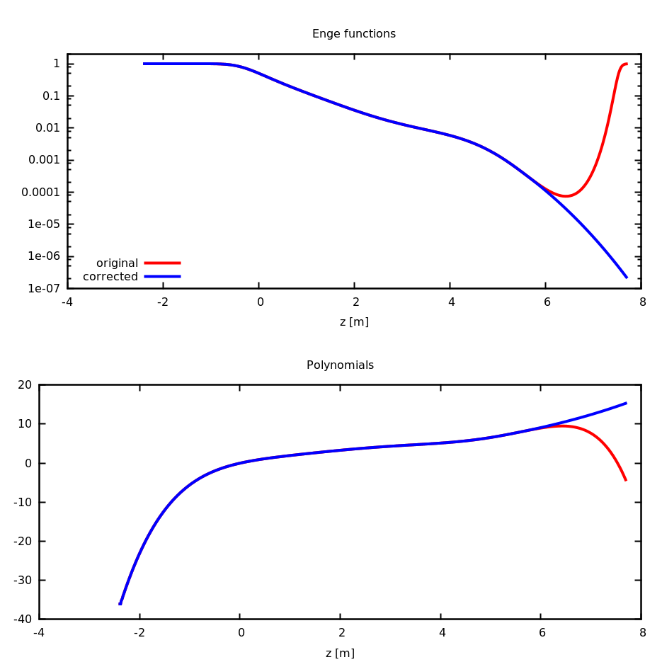
Currently, 1DProfile1 field maps are only implemented for RBEND and
SBEND elements sees RBend (OPAL-t), SBend (OPAL-t) and Bend Fields from 1D Field Maps (OPAL-t).
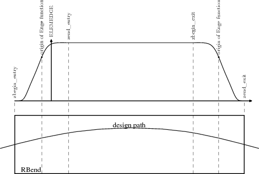
A 1DProfile1 field map has the general form shown in
Table 57. The first three lines form the file header and tell
OPAL-t how the field map data is being presented:
- Line 1
-
This tells OPAL-t what type of field file it is (
1DProfile1), the Enge coefficient order for the entrance fringe fields (\(N_{Enge\,Entrance}\)), the Enge coefficient order for the exit fringe fields (\(N_{Enge\,Exit}\)), and the gap of the magnet. - Line 2
-
The first three values on the second line are used to define the extent of the fringe fields for the entrance region of the magnet. This can be done two different ways as will be described below see 1DProfile1 Type 1 for Bend Magnet and 1DProfile1 Type 2 for Bend Magnet. The fourth value on line 2 is not currently used (but must still be present).
- Line 3
-
The first three values on the third line are used to define the extent of the fringe fields for the exit region of the magnet. This can be done two different ways as will be described below see 1DProfile1 Type 1 for Bend Magnet and 1DProfile1 Type 2 for Bend Magnet. The fourth value on line 3 is not currently used (but must still be present).
The lines following the three header lines give the entrance region Enge coefficients from \(c_0\) to \(c_{N_{Enge\,Entrance}}\), followed by the exit region Enge coefficients from \(c_0\) to \(c_{N_{Enge\,Exit}}\).
There are two types of 1DProfile1 field map files: 1DProfile Type 1
and 1DProfile1 Type 2. The difference between the two is a small
change in how the entrance and exit fringe field regions are described.
This will be explained in 1DProfile1 Type 1 for Bend Magnet and
1DProfile1 Type 2 for Bend Magnet.
1DProfile1 |
\(N_{Enge\,Entrance}\) |
\(N_{Enge\,Exit}\) |
\(Gap\) (in cm) |
Entrance Parameter 1 (in cm) |
Entrance Parameter 2 (in cm) |
Entrance Parameter 3 |
Place Holder |
Exit Parameter 1 (in cm) |
Exit Parameter 2 (in cm) |
Exit Parameter 3 |
Place Holder |
\(c_{0\, Entrance}\) |
|||
\(c_{1\, Entrance}\) |
|||
. |
|||
. |
|||
. |
|||
\(c_{N_{Enge\,Entrance}}\) |
|||
\(c_{0\,Exit}\) |
|||
\(c_{1\,Exit}\) |
|||
. |
|||
. |
|||
. |
|||
\(c_{N_{Enge\,Exit}}\) |
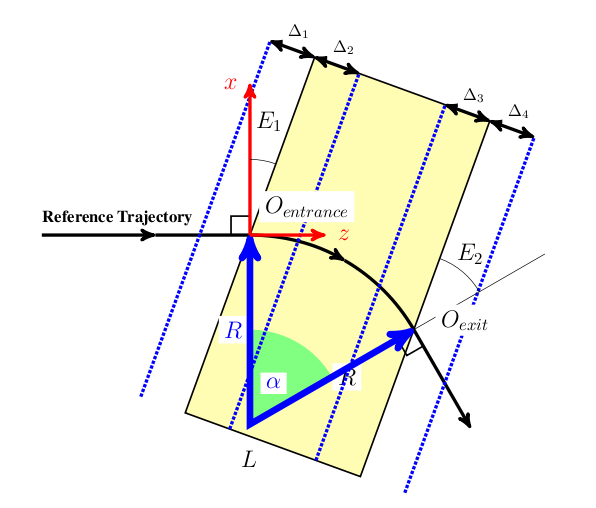
RBEND, see RBend (OPAL-t) showing the entrance and exit fringe field regions. \(\Delta_{1}\) is the perpendicular distance in front of the entrance edge of the magnet where the magnet fringe fields are non-negligible. \(\Delta_{2}\) is the perpendicular distance behind the entrance edge of the magnet where the entrance Enge function stops being used to calculate the magnet field. The reference trajectory entrance point is indicated by \(O_{entrance}\). \(\Delta_{3}\) is the perpendicular distance in front of the exit edge of the magnet where the exit Enge function starts being used to calculate the magnet field. (In the region between \(\Delta_{2}\) and \(\Delta_{3}\) the field of the magnet is a constant value.) \(\Delta_{4}\) is the perpendicular distance after the exit edge of the magnet where the magnet fringe fields are non-negligible. The reference trajectory exit point is indicated by \(O_{exit}\)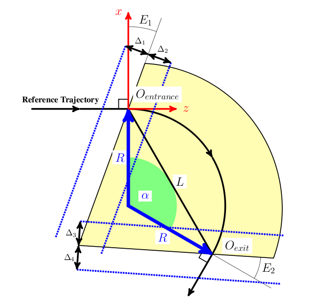
SBEND, see SBend (OPAL-t)) showing the entrance and exit fringe field regions. \(\Delta_{1}\) is the perpendicular distance in front of the entrance edge of the magnet where the magnet fringe fields are non-negligible. \(\Delta_{2}\) is the perpendicular distance behind the entrance edge of the magnet where the entrance Enge function stops being used to calculate the magnet field. The reference trajectory entrance point is indicated by \(O_{entrance}\). \(\Delta_{3}\) is the perpendicular distance in front of the exit edge of the magnet where the exit Enge function starts being used to calculate the magnet field. (In the region between \(\Delta_{2}\) and \(\Delta_{3}\) the field of the magnet is a constant value.) \(\Delta_{4}\) is the perpendicular distance after the exit edge of the magnet where the magnet fringe fields are non-negligible. The reference trajectory exit point is indicated by \(O_{exit}\).B.12.1. 1DProfile1 Type 1 for Bend Magnet
A 1DProfile1 Type 1 field map is the same 1DProfile1 field map found
in versions of OPAL previous to OPAL OPALversion1.2.0 .
Figure 45 and Figure 46 illustrate the fringe field
regions for an RBEND and an SBEND element. Referring to the general
field map file shown in Table 57, the values on lines 2 and 3
are given by:
The value of \(Entrance\,Parameter\,2\) can be any value. OPAL only cares about the relative differences between parameters. Also note that, internally, the origins of the entrance and exit Enge functions correspond to the reference trajectory entrance and exit points see Figure 45 and Figure 46.
Internally, OPAL reads in a 1DProfile Type 1 map and uses the
provided parameters to calculate the values of:
These values, combined with the entrance fringe field Enge coefficients
\(c_0\) through \(c_{N_{Enge_Entrance}}\) and exit
fringe field Enge coefficients \(c_0\) through
\(c_{N_{Enge_Exit}}\), allow OPAL to find field values
anywhere within the magnet. (Again, note that a 1DProfile Type 1 map
always places the entrance Enge function origin at the entrance point of
the reference trajectory and the exit Enge function origin at the exit
point of the reference trajectory.)
1DProfile1 6 7 3.0
-6.0 -2.0 2.0  1000
24.0 28.0 32.0 0
  0.00000e+00
  4.36222e-06
  8.83270e-06
  + 9 lines
  1.32490e-05
  1.73710e-05
  2.18598e-05
A 1D field map describing the fringe field of an element using 7 Enge
coefficients for the entrance fringe field and 8 Enge coefficients for
the exit fringe field (polynomial order 6 and 7 respectively). The
element has a gap height of 3.0 cm, and a length of 30.0 cm. The entrance
fringe field is non-negligible from 4.0 cm in front of the magnet’s
entrance edge and reaches the core strength at 4.0 cm behind the entrance
edge of the magnet. (The entrance edge position is given by the
element’s ELEMEDGE attribute.) The exit fringe field region begins
4.0 cm in front of the exit edge of the magnet and is non-negligible
4.0 cm after the exit edge of the magnet. The value 1000 at the end of
line 2 and 0 at the end of line 3 do not have any meaning.
B.12.2. 1DProfile1 Type 2 for Bend Magnet
The 1DProfile1 Type 2 field map file format was introduced in OPAL
OPALversion1.2.0 to allow for more flexibility when defining the
Enge functions for the entrance and exit fringe fields. Specifically, a
1DProfile1 Type 2 map does not contain any information about the
length of the magnet. Instead, that value is set using the element’s L
attribute. In turn, this allows us the freedom to make slight changes to
how the parameters on lines 2 and 3 of the field map file shown in
Table 57 are defined. Now
The other parameters are defined the same as before:
As before, internally, OPAL reads in a 1DProfile Type 2 map and uses
the provided parameters to calculate the values of:
These values, combined with the length of the magnet, L ( set by the
element attribute) and the entrance fringe field Enge coefficients
\(c_0\) through \(c_{N_{Enge_Entrance}}\) and exit
fringe field Enge coefficients \(c_0\) through
\(c_{N_{Enge_Exit}}\), allow OPAL to find field values
anywhere within the magnet.
The 1DProfile1 Type 2 field map file format has two main advantages:
-
The Enge function origins can be adjusted to more accurately model a magnet’s fringe fields as they are no longer fixed to the entrance and exit points of the reference trajectory.
-
Two magnets with the same fringe fields, but different lengths, can be modeled with a single
1DProfile Type 2field map file rather than two separate files.
1DProfile1 6 7 3.0
-6.0 -2.0 2.0 0
-2.0  2.0 6.0 0
  0.00000e+00
  4.36222e-06
  8.83270e-06
  + 9 lines
  1.32490e-05
  1.73710e-05
  2.18598e-05
A 1D field map describing the fringe field of an element using 7 Enge coefficients for the entrance fringe field and 8 Enge coefficients for the exit fringe field (polynomial order 6 and 7 respectively). The element has a gap height of 3.0 cm. The entrance fringe field is non-negligible from 4.0 cm in front of the magnet’s entrance edge and reaches the core strength at 4.0 cm behind the entrance edge of the magnet. The exit fringe field region begins 4.0 cm in front of the exit edge of the magnet and is non-negligible 4.0 cm after the exit edge of the magnet. The value 0 at the end of line 2 and 0 at the end of line 3 do not have any meaning. The entrance Enge function origin is 2.0 cm in front (upstream) of the magnet’s entrance edge. The exit Enge function origin is 2.0 cm behind (downstream of) the exit edge of the magnet.
B.13. 2DElectroStatic
2DElectroStatic XZ
-3.0 51.0 4999
0.0 2.0 199
  0.00000e+00  0.00000e+00
  4.36222e-06  0.00000e+00
  8.83270e-06  0.00000e+00
  + 999994 lines
  1.32490e-05  0.00000e+00
  1.73710e-05  0.00000e+00
  2.18598e-05  0.00000e+00
A 2D field map describing an electrostatic field using 5000 grid points
in the longitudinal direction times 200 grid points in the radial
direction. The field between the grid points is calculated using
bi-linear interpolation. The field is non-negligible from -3.0 cm to
51.0 cm relative to ELEMEDGE and the 200 grid points in the radial
direction span the distance from 0.0 cm to 2.0 cm. The field values are
ordered in XZ orientation, so the index in the longitudinal direction
changes fastest and therefore \(E_z\) values are stored in the
first column and \(E_r\) values in the second
see Field Map Orientation. OPAL-t normalizes the field so that
\(\max(|E_{z, \text{ on axis}}|) = 1\mathrm{MV/m}\).
2DElectroStatic |
Orientation (XZ or ZX) |
TRUE | FALSE (optional) |
\(z_{start}\) (or \(r_{start}\)) (in cm) |
\(z_{end}\) (or \(r_{end}\)) (in cm) |
\(N_{z}\) (or \(N_{r}\)) |
\(r_{start}\) (or \(z_{start}\)) (in cm) |
\(r_{end}\) (or \(z_{end}\)) (in cm) |
\(N_{r}\) (or \(N_{z}\)) |
\(E_{z,\,1}\) (or \(E_{r,\,1}\)) (MV/m) |
\(E_{r,\,1}\) (or \(E_{z,\,1}\)) (MV/m) |
|
\(E_{z,\,2}\) (or \(E_{r,\,2}\)) (MV/m) |
\(E_{r,\,2}\) (or \(E_{z,\,2}\)) (MV/m) |
|
. |
||
. |
||
. |
||
\(E_{z,\,N}\) (or \(E_{r,\,N}\)) (MV/m) |
\(E_{r,\,N}\) (or \(E_{z,\,N}\)) (MV/m) |
A 2DElectroStatic field map has the general form shown in
Table 58. The first three lines form the file header and
tell OPAL-t how the field map data is being presented:
- Line 1
-
This tells OPAL-t what type of field file it is (
2DElectroStatic) and the field orientation see Field Map Orientation. - Line 2
-
This gives the extent of the field map and how many grid spacings there are in the fastest changing index direction see Field Map Orientation.
- Line 3
-
This gives the extent of the field map and how many grid spacings there are in the slowest changing index direction (see Field Map Orientation.
The lines following the header give the 2D field map grid values from \(1\) to \(N = (N_{z} + 1) \times (N_{r} + 1)\). The order of these depend on the field orientation see Field Map Orientation and can be one of two formats:
- If Orientation = XZ
-
\(E_{z}\) (MV/m) \(E_{r}\) (MV/m)
- If Orientation = ZX
-
\(E_{r}\) (MV/m) \(E_{z}\) (MV/m)
B.14. 2DMagnetoStatic
2DMagnetoStatic ZX
0.0 2.0 199
-3.0 51.0 4999
  0.00000e+00  0.00000e+00
  0.00000e+00  4.36222e-06
  0.00000e+00  8.83270e-06
  + 999994 lines
  0.00000e+00  1.32490e-05
  0.00000e+00  1.73710e-05
  0.00000e+00  2.18598e-05
A 2D field map describing a magnetostatic field using 5000 grid points
in the longitudinal direction times 200 grid points in the radial
direction. The field between the grid points is calculated using
bi-linear interpolation. The field is non-negligible from -3.0 cm to
51.0 cm relative to ELEMEDGE and the 200 grid points in the radial
direction span the distance from 0.0 cm to 2.0 cm. The field values are
ordered in the ZX orientation, so the index in the radial direction
changes fastest and therefore \(B_r\) values are stored in the
first column and \(B_z\) values in the second
see Field Map Orientation. OPAL-t normalizes the field so that
\(\max(|B_{z,\text{ on axis}}|) = {1}{T}\).
2DMagnetoStatic |
Orientation (XZ or ZX) |
TRUE | FALSE (optional) |
\(z_{start}\) (or \(r_{start}\)) (in cm) |
\(z_{end}\) (or \(r_{end}\)) (in cm) |
\(N_{z}\) (or \(N_{r}\)) |
\(r_{start}\) (or \(z_{start}\)) (in cm) |
\(r_{end}\) (or \(z_{end}\)) (in cm) |
\(N_{r}\) (or \(N_{z}\)) |
\(B_{z,\,1}\) (or \(B_{r,\,1}\)) (T) |
\(B_{r,\,1}\) (or \(B_{z,\,1}\)) (T) |
|
\(B_{z,\,2}\) (or \(B_{r,\,2}\)) (T) |
\(B_{r,\,2}\) (or \(B_{z,\,2}\)) (T) |
|
. |
||
. |
||
. |
||
\(B_{z,\,N}\) (or \(B_{r,\,N}\)) (T) |
\(B_{r,\,N}\) (or \(B_{z,\,N}\)) (T) |
A 2MagnetoStatic field map has the general form shown in
Table 59. The first three lines form the file header and
tell OPAL-t how the field map data is being presented:
- Line 1
-
This tells OPAL-t what type of field file it is (
2DMagnetoStatic) and the field orientation see Field Map Orientation. - Line 2
-
This gives the extent of the field map and how many grid spacings there are in the fastest changing index direction see Field Map Orientation.
- Line 3
-
This gives the extent of the field map and how many grid spacings there are in the slowest changing index direction (see Field Map Orientation.
The lines following the header give the 2D field map grid values from \(1\) to \(N = (N_{z} + 1) \times (N_{r} + 1)\). The order of these depend on the field orientation see Field Map Orientation and can be one of two formats:
- If Orientation = XZ
-
\(B_{z}\) (T) \(B_{r}\) (T)
- If Orientation = ZX
-
\(B_{r}\) (T) \(B_{z}\) (T)
B.15. 2DDynamic
2DDynamic XZ
-3.0 51.0 4121
1498.953425154
0.0 1.0 75
  0.00000e+00  0.00000e+00  0.00000e+00  0.00000e+00
  4.36222e-06  0.00000e+00  0.00000e+00  4.36222e-06
  8.83270e-06  0.00000e+00  0.00000e+00  8.83270e-06
  + 313266 lines
  1.32490e-05  0.00000e+00  0.00000e+00  1.32490e-05
  1.73710e-05  0.00000e+00  0.00000e+00  1.73710e-05
  2.18598e-05  0.00000e+00  0.00000e+00  2.18598e-05
A 2D field map describing a dynamic field oscillating with a frequency
of 1498.953425154MHz. The field map provides 4122 grid points in the
longitudinal direction times 76 grid points in radial direction. The
field between the grid points is calculated with a bi-linear
interpolation. The field is non-negligible between -3.0 cm and 51.0 cm
relative to ELEMEDGE and the 76 grid points in radial direction span
the distance from 0.0 cm to 1.0 cm. The field values are ordered in the XZ
orientation, so the index in the longitudinal direction changes fastest
and therefore \(E_z\) values are stored in the first column
and \(E_r\) values in the second. The third column contains
the electric field magnitude, \(|E|\), and is not used (but
must still be included). The fourth column is \(H_{\phi}\) in
A/m. The third and fourth columns are always the same and do not depend
on the field orientation see Field Map Orientation. OPAL-t
normalizes the field so that
\(\max(|E_{z,\text{ on axis}}|) = 1\mathrm{MV/m}\).
2DDynamic |
Orientation (XZ or ZX) |
TRUE | FALSE (optional) |
|
\(z_{start}\) (or \(r_{start}\)) (in cm) |
\(z_{end}\) (or \(r_{end}\)) (in cm) |
\(N_{z}\) (or \(N_{r}\)) |
|
\(Frequency\) (in MHz) |
|||
\(r_{start}\) (or \(z_{start}\)) (in cm) |
\(r_{end}\) (or \(z_{end}\)) (in cm) |
\(N_{r}\) (or \(N_{z}\)) |
|
\(E_{z,\,1}\) (or \(E_{r,\,1}\)) (MV/m)) |
\(E_{r,\,1}\) (or \(E_{z,\,1}\)) (MV/m) |
\(|E_1|\) (MV/m) |
\(H_{\phi,\,1}\) (A/m) |
\(E_{z,\,2}\) (or \(E_{r,\,2}\)) (MV/m)) |
\(E_{r,\,2}\) (or \(E_{z,\,2}\)) (MV/m) |
\(|E_2|\) (MV/m) |
\(H_{\phi,\,2}\) (A/m) |
. |
|||
. |
|||
. |
|||
\(E_{z,\,N}\) (or \(E_{r,\,N}\)) (MV/m)) |
\(E_{r,\,N}\) (or \(E_{z,\,N}\)) (MV/m) |
latexmath:[$ |
E_N |
A 2DDynamic field map has the general form shown in Table 60.
The first four lines form the file header and tell OPAL-t how the
field map data is being presented:
- Line 1
-
This tells OPAL-t what type of field file it is (
2DDynamic) and the field orientation see Field Map Orientation. - Line 2
-
This gives the extent of the field map and how many grid spacings there are in the fastest changing index direction see Field Map Orientation.
- Line 3
-
Field frequency.
- Line 4
-
This gives the extent of the field map and how many grid spacings there are in the slowest changing index direction see Field Map Orientation.
The lines following the header give the 2D field map grid values from \(1\) to \(N= (N_{z} + 1) \times (N_{r} + 1)\). The order of these depend on the field orientation see Field Map Orientation and can be one of two formats:
- If Orientation = XZ
-
\(E_{z}\) (MV/m) \(E_{r}\) (MV/m) \(|E|\) (MV/m) \(H_{\phi}\) (A/m)
- If Orientation = ZX
-
\(E_{r}\) (MV/m) \(E_{z}\) (MV/m) \(|E|\) (MV/m) \(H_{\phi}\) (A/m)
The third item (the field magnitude) on each data line is not used by OPAL-t, but must be there.
B.16. 3DMagnetoStatic
3DMagnetoStatic
-1.5 1.5 227
-1.0 1.0 151
-3.0 51.0 4121
0.00e+00 0.00e+00 0.00e+00
0.00e+00 4.36e-06 0.00e+00
0.00e+00 8.83e-06 0.00e+00
+ 142'852'026 lines
0.00e+00 1.32e-05 0.00e+00
0.00e+00 1.73e-05 0.00e+00
0.00e+00 2.18e-05 0.00e+00
A 3D field map describing a magnetostatic field. The field map provides
4122 grid points in z-direction times 228 grid points in x-direction and
152 grid points in y-direction. The field between the grid points is
calculated with a tri-linear interpolation. The field is non-negligible
between -3.0 cm to 51.0 cm relative to ELEMEDGE, the 228 grid points in
x-direction range from -1.5 cm to 1.5 cm and the 152 grid points in
y-direction range from -1.0 cm to 1.0 cm relative to the design path. The
field values are ordered such that the index in z-direction changes
fastest, then the index in y-direction while the index in x-direction
changes slowest. The columns correspond to \(B_x\),
\(B_y\) and \(B_z\).
3DMagnetoStatic |
TRUE | FALSE (optional) |
|
\(x_{start}\) (in cm) |
\(x_{end}\) (in cm) |
\(N_{x}\) |
\(y_{start}\) (in cm) |
\(y_{end}\) (in cm) |
\(N_{y}\) |
\(z_{start}\) (in cm) |
\(z_{end}\) (in cm) |
\(N_{z}\) |
\(B_{x,\,1}\) (A/m) |
\(B_{y,\,1}\) (A/m) |
\(B_{z,\,1}\) (A/m) |
\(B_{x,\,2}\) (A/m) |
\(B_{y,\,2}\) (A/m) |
\(B_{z,\,2}\) (A/m) |
. |
||
. |
||
. |
||
\(B_{x,\,N}\) (A/m) |
\(B_{y,\,N}\) (A/m) |
\(B_{z,\,N}\) (A/m) |
A 3DMagnetoStatic field map has the general form shown in
Table 61. The first five lines form the file header and
tell OPAL-t how the field map data is being presented:
- Line 1
-
This tells OPAL-t what type of field file it is (
3DMagnetoStatic). - Line 3
-
This gives the extent of the field map and how many grid spacings there are in the slowest changing index direction.
- Line 4
-
This gives the extent of the field map and how many grid spacings there are in the next fastest changing index direction.
- Line 5
-
This gives the extent of the field map and how many grid spacings there are in the fastest changing index direction.
The lines following the header give the 3D field map grid values from \(1\) to \(N= (N_{z} + 1) \times (N_{y} + 1) \times (N_{x} + 1)\).
B.17. 3DMagnetoStatic_Extended
3DMagnetoStatic_Extended
-9.9254 9.9254 133
-2.0 1.0 15
-22.425 47.425 465
 -8.10970000e-05
 -8.38540000e-05
 -8.64960000e-05
+ 62'438 lines
 -8.64960000e-05
 -8.38540000e-05
 -8.10970000e-05
A 3D field map describing a magnetostatic field on the mid-plane. The
field map provides 466 grid points in z-direction times 134 grid points
in x-direction. The field is non-negligible between -22.425 cm to
47.425 cm relative to ELEMEDGE, the 134 grid points in x-direction
range from -9.9254cm to 9.9254cm. The field should be integrated using
Maxwell’s equations from the mid-plane to 2.0 cm using 16 grid points.
The mid-plane is regarded as a perfect magnetic conductor (PMC) i.e. the
magnetic field on the mid-plane has no tangential component. This leads
to a symmetry where the perpendicular component is mirrored whereas the
tangential component is anti-parallel. Instead of integrating the field
from the mid-plane to -2.0 cm and 1.0 cm we only integrate it to +2.0 cm
and store only the upper half of the field map. For positions
\(R(x,\;-y,\;z)\) with \(y > 0.0\) the correct field
can then be derived from the \(R(x,\;y,\;z)\).
TRUE | FALSE (optional) |
||
\(x_{start}\) (in cm) |
\(x_{end}\) (in cm) |
\(N_{x}\) |
\(y_{start}\) (in cm) |
\(y_{end}\) (in cm) |
\(N_{y}\) |
\(z_{start}\) (in cm) |
\(z_{end}\) (in cm) |
\(N_{z}\) |
\(B_{y,\,1}\) (T) |
||
\(B_{y,\,2}\) (T) |
||
. |
||
. |
||
. |
||
\(B_{y,\,N}\) (T) |
A 3DMagnetoStatic_Extended field map has the general form shown in
Table 62. The first four lines form the file
header and tell OPAL-t how the field map data is being presented:
- Line 1
-
This tells OPAL-t what type of field file it is (
3DMagnetoStatic_Extended). - Line 2
-
This gives the extent of the field map and how many grid spacings there are in the slowest changing direction.
- Line 3
-
This gives the extent of the field map and how many grid spacings there are in the next fastest changing direction.
- Line 4
-
This gives the extent of the field map and how many grid spacings there are in the fastest changing direction.
The lines following the header give the 3D field map grid values from \(1\) to \(N= (N_{z} + 1) \times (N_{x} + 1)\). The order of these depend on the field orientation see Field Map Orientation and can currently only be the format shown in Table 62.
B.18. 3DDynamic
3DDynamic
1498.9534
-1.5 1.5 227
-1.0 1.0 151
-3.0 51.0 4121
0.00e+00 0.00e+00 0.00e+00 0.00e+00 0.00e+00 0.00e+00
4.36e-06 0.00e+00 4.36e-06 0.00e+00 4.36e-06 0.00e+00
8.83e-06 0.00e+00 8.83e-06 0.00e+00 8.83e-06 0.00e+00
+ 142'852'026 lines
1.32e-05 0.00e+00 1.32e-05 0.00e+00 1.32e-05 0.00e+00
1.73e-05 0.00e+00 1.73e-05 0.00e+00 1.73e-05 0.00e+00
2.18e-05 0.00e+00 2.18e-05 0.00e+00 2.18e-05 0.00e+00
A 3D field map describing a dynamic field oscillating with 1.4989534.
The field map provides 4122 grid points in z-direction times 228 grid
points in x-direction and 152 grid points in y-direction. The field
between the grid points is calculated with a tri-linear interpolation.
The field is non-negligible between -3.0 cm to 51.0 cm relative to
ELEMEDGE, the 228 grid points in x-direction range from -1.5 cm to
1.5 cm and the 152 grid points in y-direction range from -1.0 cm to 1.0 cm
relative to the design path. The field values are ordered such that the
index in z-direction changes fastest, then the index in y-direction
while the index in x-direction changes slowest. The columns correspond
to \(E_x\), \(E_y\), \(E_z\),
\(H_x\), \(H_y\) and \(H_z\). OPAL-t
normalizes the field so that
\(\max(|E_{z,\text{ on axis}}|) = 1\mathrm{MV/m}\).
3DDynamic |
TRUE | FALSE (optional) |
||||
\(Frequency\) (in MHz) |
|||||
\(x_{start}\) (in cm) |
\(x_{end}\) (in cm) |
\(N_{x}\) |
|||
\(y_{start}\) (in cm) |
\(y_{end}\) (in cm) |
\(N_{y}\) |
|||
\(z_{start}\) (in cm) |
\(z_{end}\) (in cm) |
\(N_{z}\) |
|||
\(E_{x,\,1}\) (MV/m)) |
\(E_{y,\,1}\) (MV/m) |
\(E_{z,\,1}\) (MV/m) |
\(H_{x,\,1}\) (A/m) |
\(H_{y,\,1}\) (A/m) |
\(H_{z,\,1}\) (A/m) |
\(E_{x,\,2}\) (MV/m)) |
\(E_{y,\,2}\) (MV/m) |
\(E_{z,\,2}\) (MV/m) |
\(H_{x,\,2}\) (A/m) |
\(H_{y,\,2}\) (A/m) |
\(H_{z,\,2}\) (A/m) |
. |
|||||
. |
|||||
. |
|||||
\(E_{x,\,N}\) (MV/m)) |
\(E_{y,\,N}\) (MV/m) |
\(E_{z,\,N}\) (MV/m) |
\(H_{x,\,N}\) (A/m) |
\(H_{y,\,N}\) (A/m) |
\(H_{z,\,N}\) (A/m) |
A 3DDynamic field map has the general form shown in Table 63.
The first five lines form the file header and tell OPAL-t how the
field map data is being presented:
- Line 1
-
This tells OPAL-t what type of field file it is (
3DDynamic). - Line 2
-
Field frequency.
- Line 3
-
This gives the extent of the field map and how many grid spacings there are in the slowest changing index direction.
- Line 4
-
This gives the extent of the field map and how many grid spacings there are in the next fastest changing index direction.
- Line 5
-
This gives the extent of the field map and how many grid spacings there are in the fastest changing index direction.
The lines following the header give the 3D field map grid values from \(1\) to \(N= (N_{z} + 1) \times (N_{y} + 1) \times (N_{x} + 1)\).
B.19. References
[66] J. E. Spencer and H. A. Enge, Split-pole magnetic spectrograph for precision nuclear spectroscopy, Nucl. Instrum. Methods 49, 181 (1967).
[67] J. H. Billen and L. M. Young, Poisson superfish, Tech. Rep. LA-UR-96-1834, Los Alamos National Laboratory (2004).
Appendix C: OPAL - MADX Conversion Guide
We note with \(\alpha\),\(\beta\) and \(\gamma\) the Twiss parameters.
| Quantity | MADX |
Conversion | OPAL-Output | ||||
|---|---|---|---|---|---|---|---|
Momenta |
\(\bar{p}_{x}\) |
[rad] |
\(\bar{p}_{x}\)[\(\beta\gamma\)] |
= |
\(\left(\bar{p}_{x}\left[\text{rad}\right]\right)\cdot\left(\beta\gamma\right)\) |
\(\bar{p}_{x}\) |
[\(\beta\gamma\)] |
Correlation of \(\bar{x}\),\(\bar{p}_{x}\) |
\(\delta\) |
[1] |
\(\delta\) |
= |
\(\left(\sigma_{x p_{x}}\left[\text{m }\text{rad}\right]\right)/\left(\left(\bar{p}_{x}\left[\text{rad}\right]\right)\cdot\left( \bar{x}\left[\text{m}\right]\right)\right)\) |
\(\delta\) |
[1] |
= |
\(\left(\sigma_{x p_{x}}\left[\text{m }\text{rad}\right]\right)/\sqrt{\left(\sigma_{x}\left[\text{m}^{2}\right]\right)\cdot\left(\sigma_{ p_{x}}\left[\text{rad}^{2}\right]\right)}\) |
||||||
Emittance |
\(\epsilon_{x}\) |
[m rad] |
\(\epsilon_{x}\)[m \(\beta\gamma\)] |
= |
\(\sqrt{\left( \bar{p}_{x}\left[ \beta\gamma \right] \right) ^{2} \cdot \left(\bar{x}\left[\text{m}\right]\right)^{2} - \left(\delta \cdot \left(\bar{x}\left[\text{m}\right]\right) \cdot \left(\bar{p}_{x}\left[\beta\gamma\right]\right)\right)^{2}} \) |
\(\epsilon_{x}\) |
[m \(\beta\gamma\)] |
= |
\(\sqrt{\left( \sigma_{{p}_{x}}\left[ \left(\beta\gamma\right)^{2} \right] \right)\cdot \left(\sigma_{x}\left[\text{m}^{2}\right]\right) - \left(\delta \cdot \sqrt{\left(\sigma_{x}\left[\text{m}^{2}\right]\right)\cdot\left(\sigma_{p_{x}} \left[\left(\beta\gamma\right)^{2}\right]\right)}\right)^{2}} \) |
||||||
= |
\(\sqrt{\left( \sigma_{{p}_{x}}\left[ \left(\beta\gamma\right)^{2} \right] \right)\cdot \left(\sigma_{x}\left[\text{m}^{2}\right]\right) - \left(\sigma_{x p_{x}}\left[\text{m} ~\beta\gamma\right]\right)^{2}} \) |
||||||
Twiss Parameter \(\alpha\) |
\(\alpha\) |
[1] |
\(\alpha\left[1\right]\) |
= |
\(-\delta\cdot\left(\bar{x}\left[\text{m}\right]\right)\cdot\left(\bar{p}_{x}\left[\beta\gamma\right]\right)/\left(\epsilon_{x}\left[\text{m}~\beta\gamma\right]\right)\) |
\(\alpha_{T}\) |
[1] |
= |
\(-\delta\cdot\sqrt{\left(\sigma_{x}\left[\text{m}^{2}\right]\right)\cdot\left(\sigma_{ p_{x}}\left[\left(\beta\gamma\right)^{2}\right]\right)}/\left(\epsilon_{x}\left[\text{m}~\beta\gamma\right]\right)\) |
||||||
Twiss Parameter \(\beta_{T}\) |
\(\beta_{T}\) |
[m/rad] |
\(\beta_{T}\left[\text{m}/\beta\gamma\right]\) |
= |
\(\left(\bar{x}\left[\text{m}\right]\right)^{2}/\left(\epsilon_{x}\left[\text{m}~\beta\gamma\right] \right)\) |
\(\beta_{T}\) |
[m/\(\beta\gamma\)] |
= |
\(\left(\sigma_{x}\left[\text{m}^{2}\right]\right)/\left(\epsilon_{x}\left[\text{m}~\beta\gamma\right] \right)\) |
||||||
Twiss Parameter \(\gamma_{T}\) |
\(\gamma_{T}\) |
[rad/m] |
\(\gamma_{T}\left[\beta\gamma/\text{m}\right]\) |
= |
\(\left(\bar{p}_{x}\left[\beta\gamma\right]\right)^{2}/\left(\epsilon_{x}\left[\text{m}~\beta\gamma\right]\right)\) |
\(\gamma_{T}\) |
[\(\beta\gamma\)/m] |
= |
\(\left(\sigma_{p_{x}}\left[\left(\beta\gamma\right)^{2}\right]\right)/\left(\epsilon_{x}\left[\text{m}~\beta\gamma\right]\right)\) |
||||||
Focusing strength |
\(k_{1}\) |
\(\left[\text{m}^{-2}\right]\) |
\(k_{1}\left[\text{T}/\text{m}\right]\) |
= |
\(\left(k_{1}\left[\text{m}^{-2}\right]\right)\cdot\left(\text{B}\rho\left[\text{T m}\right]\right)\) |
\(k_{1}\) |
\(\left[\text{T}/\text{m}\right]\) |
| Quantity | MADX |
Conversion | OPAL-Input |
||||
|---|---|---|---|---|---|---|---|
Element Position |
|
\(\left[\text{m}\right]\) |
|
= |
(Center of the element) - (Length of the element)/2 |
|
\(\left[\text{m}\right]\) |
Center of the element |
Begin of the element |
||||||
| Quantity | OPAL-Output |
Conversion | OPAL-Input |
||||
|---|---|---|---|---|---|---|---|
Momenta |
\(\bar{p}_{x}\) |
\(\left[\beta\gamma\right]\) |
\(p_{x}\left[\text{eV}\right]\) |
= |
\(m_{p}\cdot10^{9}\cdot\left(\sqrt{\left(\bar{p}_{x}\left[\beta\gamma\right]\right)^{2} +1}-1\right)\) |
\(\bar{p}_{x}\) |
[eV] |
Appendix D: Auto-phasing Algorithm
D.1. Standing Wave Cavity
In OPAL-t the elements are implemented as external fields that are read in from a file. The fields are described by a 1D, 2D or 3D sampling (equidistant or non-equidistant). To get the actual field at any position a linear interpolation multiplied by \(\cos(\omega t + \varphi)\), where \(\omega\) is the frequency and \(\varphi\) is the lag. The energy gain of a particle then is
To maximize the energy gain we have to take the derivative with respect to the lag, \(\varphi\) and set the result to zero:
Thus to get the maximum energy the lag has to fulfill
where
and
Between two sampling points we assume a linear correlation between the electric field and position respectively between time and position. The products in the integrals between two sampling points can be expanded and solved analytically. We then find
and
where
It remains to find the progress of time with respect to the position. In OPAL this is done iteratively starting with
K[i] = K[i-1] + (z[i] - z[0]) * q * V;
b[i] = sqrt(1. - 1. / ((K[i] - K[i-1]) / (2.*m*c^2) + 1)^2);
t[i] = t[0] + (z[i] - z[0]) / (c * b[i])
By doing so we assume that the kinetic energy, K, increases linearly and proportional to the maximal voltage. With this model for the progress of time we can calculate \(\varphi\) according to Lag rule. Next a better model for the kinetic Energy can be calculated using
K[i] = K[i-1] + q \(\Delta\)z[i](cos(\(\varphi\))(Ez[i-1](\(\Gamma_{21}\)[i] - \(\Gamma_{22}\)[i]) + Ez[i]\(\Gamma_{22}\)[i])
\(\,\,\)- sin(\(\varphi\))(Ez[i-1](\(\Gamma_{11}\)[i] - \(\Gamma_{12}\)[i]) + Ez[i]\(\Gamma_{12}\)[i])).
With the updated kinetic energy the time model and finally a new \(\varphi\), that comes closer to the actual maximal kinetic energy, can be obtained. One can iterate a few times through this cycle until the value of \(\varphi\) has converged.
D.2. Traveling Wave Structure
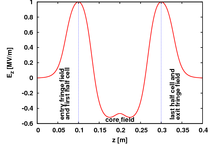
Auto phasing in a traveling wave structure is just slightly more complicated. The field of this element is composed of a standing wave entry and exit fringe field and two standing waves in between, see Figure 47.
where \(s\) is the cell length. Instead of one sum as in Gamma 1 and Gamma 2 there are four sums with different numbers of summands.
D.2.1. Example
FINLB02_RAC: TravelingWave, L=2.80, VOLT=14.750*30/31,
             NUMCELLS=40, FMAPFN="FINLB02-RAC.T7",
             ELEMEDGE=2.67066, MODE=1/3,
             FREQ=1498.956, LAG=FINLB02_RAC_lag;
For this example we find
D.2.2. Alternative Approach for Traveling Wave Structures
If \(\beta\) doesn’t change much along the traveling wave structure (ultra relativistic case) then \(t(z,\varphi)\) can be approximated by \(t(z,\varphi)=\frac{\omega}{\beta c}z + t_{0}\). For the example from above the energy gain is approximately
Here \(\beta c = 2.9886774\cdot10^8\;\text{m s}^{-2}\), \(\omega = 2\pi\cdot 1.4989534\cdot10^9\) Hz and, the cell length, \(s = 0.06\bar{6}\) m. To maximize this energy we have to take the derivative with respect to \(\varphi\) and set the result to \(0\). We split the field up into the core field, \(E_z^{(1)}\) and the fringe fields (entry fringe field plus first half cell concatenated with the exit fringe field plus last half cell), \(E_z^{(2)}\). The core fringe field is periodic with a period of \(3\,s\). We thus find
This equation is much simplified if we take into account that \(\omega / \beta c \approx 10\pi\). We then get
where we used \((z' = z + s)\)
In the last equal sign we used the fact that both functions, \(\sin(\frac{\omega}{\beta c}z)\) and \(E_z^{(1)}\) have a periodicity of \(3\cdot s\) to shift the boundaries of the integral.
Using the convolution theorem we find
where
and
Here we also used some trigonometric identities:
Appendix E: Benchmarks
E.1. OPAL-t compared with TRANSPORT & TRACE 3D
E.1.1. TRACE 3D
TRACE 3D is an interactive beam dynamics program that calculates the envelopes of a bunched beam, including linear space-change forces [68]. It provides an instantaneous beam profile diagram and delineates the transverse and longitudinal phase plane, where the ellipses are characterized by the Twiss parameters and emittances (total and unnormalized).
E.1.2. TRACE 3D Units
TRACE 3D supports the following internal coordinates and units for the three phase planes:
-
horizontal plane:
x [mm] is the displacement from the center of the beam bunch;
x’ [mrad] is the beam divergence; -
vertical plane:
y [mm] is the displacement from the center of the beam bunch;
y’ [mrad] is the beam divergence; -
longitudinal plane:
z [mm] is the displacement from the center of the beam bunch;
\(\Delta\)p/p [mrad] is the difference between the particle’s longitudinal momentum and the reference momentum of the beam bunch.
For input and output, however, z and \(\Delta\)p/p are replaced by \(\Delta\phi\) [degree] and \(\Delta\)W [keV], respectively the displacement in phase and energy. The relationships between these longitudinal coordinates are:
and
where \(\beta\) and \(\gamma\) are the relativist parameters, \(\lambda\) is the free-space wavelength of the RF and W is the kinetic energy [MeV] at the beam center. This internal conversion can be displayed using the command W (see [68] page 42).
E.1.3. TRACE 3D Input beam
In TRACE 3D, the input beam is described by the following set of parameters:
-
ER: particle rest mass [MeV/c^{2}];
-
Q: charge state (+1 for protons);
-
W: beam kinetic energy [MeV]
-
XI: beam current [mA]
-
BEAMI: array with initial Twiss parameters in the three phase planes
BEAMI = \(\alpha_x , \beta_x, \alpha_y, \beta_y, \alpha_{\phi}, \beta_{\phi} \)
The alphas are dimensionless, \(\beta_x\) and \(\beta_y\) are expressed in m/rad (or mm/mrad) and \(\beta_{\phi}\) in deg/keV;
-
EMITI: initial total and unnormalized emittances in x-x’, y-y’, and \(\Delta\phi\)-\(\Delta W\) planes.
EMITI = \(\epsilon_x , \epsilon_y, \epsilon_{\phi} \)
The transversal emittances are expressed in \(\pi\)-mm-mrad and in \(\pi\)-deg-keV the longitudinal emittance.
In this beam dynamics code, the total emittance in each phase plane is five times the RMS emittance in that plane and the displayed beam envelopes are \(\sqrt{5}\)-times their respective RMS values.
TRACE 3D Graphic Interface
An example of TRACE 3D graphic interface is shown in Figure 48.
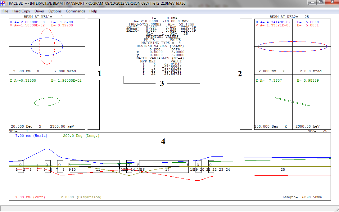
E.1.4. TRANSPORT
TRANSPORT is a computer program for first-order and second-order matrix multiplication, intended for the design of beam transport system [69]. The TRANSPORT version for Windows provides a graphic beam profile diagram, as well as a sigma matrix description of the simulated beam and line [70]. Differently from TRACE 3D, the ellipses are characterized by the sigma-matrix coefficients and the Twiss parameters and emittances (total and unnormalized) are reported as output information.
E.1.5. TRANSPORT Units
At any specified position in the system, an arbitrary charged particle is represented by a vector, whose components are positions, angles and momentum of the particle with respect to the reference trajectory. The standard units and internal coordinates in TRANSPORT are:
-
horizontal plane:
x [cm] is the displacement of the arbitrary ray with respect to the assumed central trajectory;
\(\theta\) [mrad] is the angle the ray makes with respect to the assumed central trajectory; -
vertical plane:
y [cm] is the displacement of the arbitrary ray with respect to the assumed central trajectory;
\(\phi\) [mrad] is the angle the ray makes with respect to the assumed central trajectory; -
longitudinal plane:
l [cm] is the path length difference between the arbitrary ray and the central trajectory;
\(\delta\) [%] is the fractional momentum deviation of the ray from the assumed central trajectory.
Even if TRANSPORT supports this standard set of units [cm, mrad and %]; however using card 15, the users can redefine the units (see page 99 on TRANSPORT documentation [69] for more details).
E.1.6. TRANSPORT Input beam
The input beam is described in card 1 in terms of the semi-axes of a six-dimensional erect ellipsoid beam. In terms of diagonal sigma-matrix elements, the input beam in TRANSPORT is expressed by 7 parameters:
-
\(\sqrt{\sigma_{ii}}\) [cm] represents one-half of the horizontal (i=1), vertical (i=3) and longitudinal extent (i=5);
-
\(\sqrt{\sigma_{ii}}\) [mrad] represents one-half of the horizontal (i=2), vertical (i=4) beam divergence;
-
\(\sqrt{\sigma_{66}}\) [%] represents one-half of the momentum spread;
-
p(0) is the momentum of the central trajectory [GeV/c].
If the input beam is tilted (Twiss alphas not zero), card 12 must be used, inserting the 15 correlations \(r_{ij}\) parameters among the 6 beam components. The correlation parameters are defined as following:
As explained before, with the card 15, it is possible to transform the TRANSPORT standard units in TRACE-like units. In this way, the TRACE 3D sigma-matrix for the input beam, printed out by command Z, can be directly used as input beam in TRANSPORT. An example of TRACE 3D sigma-matrix structure is shown in Figure 49.
From the sigma-matrix coefficients, TRANSPORT reports in output the Twiss parameters and the total, unnormalized emittance. Even in this case, a factor 5 is present between the emittances calculated by TRANSPORT and the corresponding RMS values.
TRANSPORT Graphic Interface
An improved version of TRANSPORT has been embedded in a new graphic shell written in C++ and is providing GUI type tools, which makes it easier to design new beam lines. A screen shot of a modern GUI Transport interface [70] is shown in Figure 50.
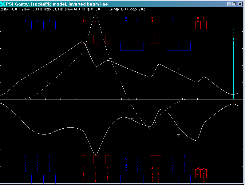
E.1.7. Comparison TRACE 3D and TRANSPORT
This study has been done following the same trend of the Regression Test in OPAL, replacing the electron beam with a same energy proton beam. Due to the different beam rigidity, the bending magnet features have been redefined with a new magnetic field.
The simulated beam transport line contains:
-
drift space (DRIFT 1): 0.250 m length;
-
bending magnet (SBEND or RBEND): 0.250 m radius of curvature;
-
drift space (DRIFT 2): 0.250 m length.
Keeping fixed the lattice structure, many similar transport lines have been tested adding entrance and exit edge angles to the bending magnet, changing the bending plane (vertical bending magnet) and direction (right or left). In all the cases, the difficulties arise from the non-achromaticity of the system and an increase in the horizontal and longitudinal emittance is expected. In addition, the coupling between these two planes has to be accurately studied.
In the following paragraph, an example of Sector Bending magnet (SBEND) simulation with entrance and exit edge angles is discussed.
Input beam
The starting simulation has been performed with TRACE 3D code. According to TRACE 3D Input beam, the simulated input beam is described by the following parameters:
ER = 938.27
W = 7
FREQ = 700
BEAMI = 0.0, 4.0,0.0, 4.0, 0.0, 0.0756
EMITI = 0.730, 0.730, 7.56
Thanks to the TRACE 3D graphic interface, the input beam can immediately be visualized in the three phase plane as shown in Figure 51.
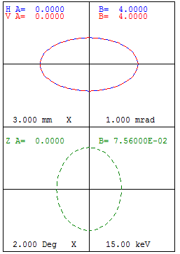
The corresponding sigma-matrix with the relative units is displayed by command Z:
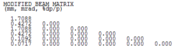
Before entering the TRACE 3D sigma-matrix coefficients in TRANSPORT, a changing in the units is required using the card 15 in the following way:
15. 1. 'MM' 0.1 ; //express in mm the horizontal and vertical beam size
15. 5. 'MM' 0.1 ; //express in mm the beam length
At this point, the TRANSPORT input beam is defined by card 1:
1.0 1.709 0.427 1.709 0.427 0.11 0.0717 0.1148 /BEAM/ ;
using exactly the same sigma-matrix coefficients of Figure 52. Other two cards must be added in order to use exactly the TRACE 3D R-matrix formalism:
16. 3. 1863.153; //proton mass, as ratio of electron mass
22. 0.05 0.0 700 0.0 /SPAC/ ; //space charge card
SBEND in TRACE 3D
The bending magnet definition in TRACE 3D requires:
| Parameter | Value | Description |
|---|---|---|
NT |
8 |
Type code for bending |
\(\alpha\) [deg] |
30 |
angle of bend in horizontal plane |
\(\rho\) [mm] |
250 |
radius of curvature of central trajectory |
n |
0 |
field-index gradient |
vf |
0 |
flag for vertical bending |
The edge angles are described with another type code and parameters which include also the fringe field. They must be added before and after the bending magnet if entrance and exit edge angles are present and if the fringe field has to be taken into account. In particular for the entrance edge angle:
| Parameter | Value | Description |
|---|---|---|
NT |
9 |
Type code for edge |
\(\beta\) [deg] |
10 |
pole-face rotation |
\(\rho\) [mm] |
250 |
radius of curvature of central trajectory |
g [mm] |
20 |
total gap of magnet |
\(K_1\) |
0.36945 |
fringe-field factor |
\(K_2\) |
0.36945 |
fringe-field factor |
A same configuration has been used for exit edge angle using \(\beta = {5}{^{\circ}}\). The beam envelopes in the three phase planes for this simulation are shown in Figure 53.
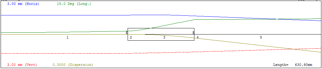
SBEND in TRANSPORT
The bending magnet definition in TRANSPORT requires:
| Parameter | Value | Description |
|---|---|---|
Card |
4 |
Type code for bending |
L [m] |
30 |
Effective length of the central trajectory |
\(B_0\) [kG] |
250 |
Central field strength |
n |
0 |
field-index gradient |
As for TRACE 3D, the edge angles are described with another card and parameters. In TRANSPORT, however, the fringe field is not automatically included with the edge angle, but it is described by a own card as reported in the Table 67.
| Parameter | Value | Description |
|---|---|---|
Card |
2 |
Type code for edge |
\(\beta\) [deg] |
10 |
pole-face rotation |
Card |
16 |
Type code for fringe field |
g [mm] |
10 |
half-gap of magnet |
\(K_1\) |
0.36945 |
fringe-field factor |
\(K_2\) |
0.36945 |
fringe-field factor |
Running the Graphic TRANSPORT version, the beam envelopes in the transverse phase planes for this simulation are shown in Figure 54.
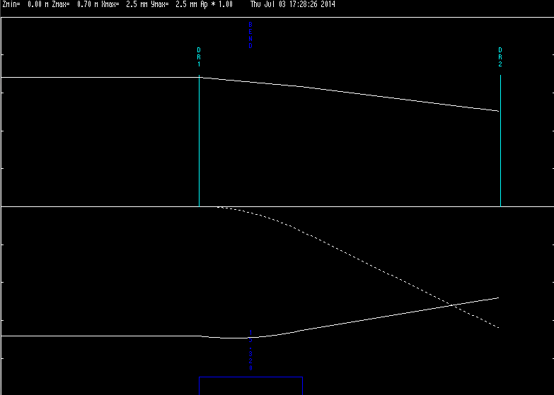
Beam size and emittance comparison
In the next table, the results of the comparison between TRACE 3D and TRANSPORT in terms of the transversal beam sizes at the end of each element in the line are summarized.
Position |
z (m) |
\(\sigma_x\) (mm) |
\(\sigma_y\) (mm) |
\(\sigma_x\) (mm) |
\(\sigma_y\) (mm) |
Input |
0.000 |
1.709 |
1.709 |
1.709 |
1.709 |
Drift 1 |
0.250 |
1.712 |
1.712 |
1.712 |
1.712 |
Edge |
0.250 |
1.712 |
1.712 |
1.712 |
1.712 |
Bend |
0.381 |
1.638 |
1.587 |
1.638 |
1.587 |
Edge |
0.381 |
1.638 |
1.587 |
1.638 |
1.587 |
Drift 2 |
0.631 |
1.206 |
1.264 |
1.206 |
1.264 |
The perfect agreement between these two codes arises immediately looking at Figure 55.
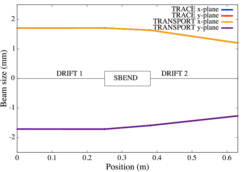
The same comparison has been performed in terms of horizontal and longitudinal emittance, both expressed in \(\pi\)-mm-mrad. While the vertical emittance remains constant and equal to the initial value (\(\epsilon_y = \) 0.730 \(\pi\)-mm-mrad) , the horizontal and longitudinal emittances are expected growing after the bending magnet. The results are reported in Table 69 and in Figure 56.
Position |
z (m) |
\(\epsilon_x\) |
\(\epsilon_z\) |
\(\epsilon_x\) |
\(\epsilon_z\) |
Input |
0 |
0.730 |
0.08 |
0.730 |
0.08 |
Drift 1 |
0.250 |
0.730 |
0.08 |
0.730 |
0.08 |
Edge |
0.250 |
0.730 |
0.08 |
0.730 |
0.08 |
Bend |
0.381 |
0.973 |
0.65 |
0.973 |
0.65 |
Edge |
0.381 |
0.973 |
0.65 |
0.973 |
0.65 |
Drift 2 |
0.631 |
0.973 |
0.65 |
0.973 |
0.65 |
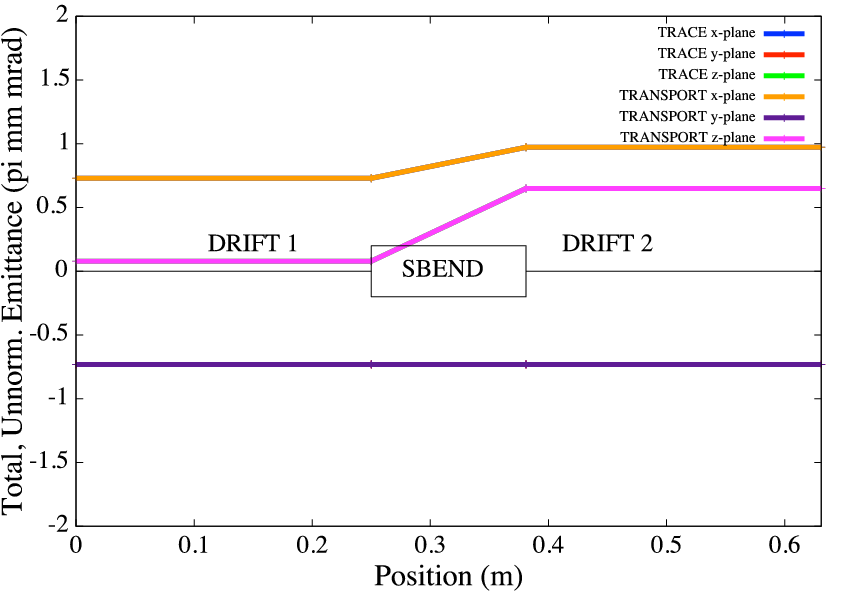
From TRACE 3D to TRANSPORT
| Parameter | Trace 3D | Transport |
|---|---|---|
Bend card |
8 |
4 |
Angle |
Input parameter [deg] |
Output information [deg] |
Magn. field |
Calculated. [T] |
Input parameter [kG] |
Radius of curv. |
Input parameter [mm] |
Output information [m] |
Field-index |
Input parameter |
Input parameter |
Effect. length |
Calculated [mm] |
Input parameter [m] |
Edge card |
9 |
2 |
Edge angle |
Input parameter [deg] |
Input parameter [deg] |
Vertical gap |
9 |
16.5 |
Gap |
Total [mm] |
Half-gap [cm] |
Fringe field card |
9 |
16.7 / 16.8 |
\(K_1\) |
Default: 0.45 |
Default: 0.5 |
\(K_2\) |
Default: 2.8 |
Default: 0 |
Bend direction |
Bend angle sign |
Coord. rotation |
Horiz. right |
Angle \(>\) 0 |
Angle \(>\) 0 |
Horiz. left |
Angle \(<\) 0 |
Card 20 |
Vertical bend |
Card 8, vf \(>\) 0 |
Card 20 |
E.1.8. Relations to OPAL-t
In OPAL, the beam dynamics approach (time integration) is hence completely different from the envelope-like supported by TRACE 3D and TRANSPORT. The three codes support different units and require diverse parameters for the input beam. A summary of their main features is reported in Table 71.
| Code | TRACE 3D | TRANSPORT | OPAL |
|---|---|---|---|
Type |
Envelope |
Envelope |
Time integration |
Input |
Twiss, Emittance |
Sigma, Momentum |
Sigma, Energy |
Units |
mm-mrad, deg-keV |
cm-rad, cm-% |
m-\(\beta\gamma\) |
E.1.9. OPAL-t Units
OPAL-t supports the following internal coordinates and units for the three phase planes:
-
horizontal plane:
X [m] horizontal position of a particle relative to the axis of the element;
PX [\(\beta_x\gamma\)] horizontal canonical momentum; -
vertical plane:
Y [m] vertical position of a particle relative to the axis of the element;
PY [\(\beta_y\gamma\)] horizontal canonical momentum; -
longitudinal plane:
Z [m] longitudinal position of a particle in floor-coordinates;
PZ [\(\beta_z\gamma\)] longitudinal canonical momentum;
E.1.10. OPAL-t Input beam
For the input beam, a GAUSS distribution type has been chosen. For
transferring the TRANSPORT (or TRACE 3D) input beam in terms of
sigma-matrix coefficients, it necessary to:
-
adjust the units: from mm to m;
-
correct for the factor \(\sqrt{5}\): from total to RMS distribution;
-
multiply for the relativistic factor \(\beta\gamma ={0.1224}\) for 7 MeV protons;
In case of the modified sigma-matrix in Figure 52, the
corresponding OPAL parameters for the GAUSS distributions are:
 T3D SIGMA                        OPAL -T
 -------------------------------------------------------
 1.7088 mm             SIGMAX  = 1.7088/sqrt(5)e-3         m
 0.4272 mrad           SIGMAPX = 0.4272/sqrt(5)*0.1224e-3
 1.7088 mm             SIGMAY  = 1.7088/sqrt(5)e-3        m
 0.4272 mrad           SIGMAPY = 0.4272/sqrt(5)*0.1224e-3
 0.1092 mm             SIGMAZ  = 0.1092/sqrt(5)e-3        m
 0.0717 %              SIGMAPZ = (0.0717*10)/sqrt(5)*0.1224e-3
At the end of this calculation, the input beam in OPAL is:
D1: DISTRIBUTION, TYPE=GAUSS,
SIGMAX = 0.7642e-03,  SIGMAPX= 0.0234e-03,  CORRX= 0.0,
SIGMAY = 0.7642e-03,  SIGMAPY= 0.0234e-03,  CORRY= 0.0,
SIGMAZ = 0.0488e-03,  SIGMAPZ= 0.0392e-03,  CORRZ= 0.0, R61= 0.0,
INPUTMOUNITS=NONE;
E.1.11. Comparison TRACE 3D and OPAL-t
In this section, the comparison between TRACE 3D and OPAL-t is
discussed starting from SBEND definition in OPAL-t. The transport
line described in Comparison TRACE 3D and TRANSPORT has been simulated in OPAL using
10.000 particles and \(10^{-11}\) s time step. The bending
magnet features of Table 64 and Table 65 have been transformed
in OPAL language as:
Bend: SBEND, ANGLE = 30.0 * Pi/180.0,
             K1=0.0,
             E1=0, E2=0,
             FMAPFN = "1DPROFILE1-DEFAULT",
             ELEMEDGE = 0.250,  // end of first drift
             DESIGNENERGY = 7E+06,  // ref energy eV
             L = 0.1294,
             GAP = 0.02;
-
SBEND without edge angles:
// Bending magnet configuration:
K1=0.0,
E1=0, E2=0,
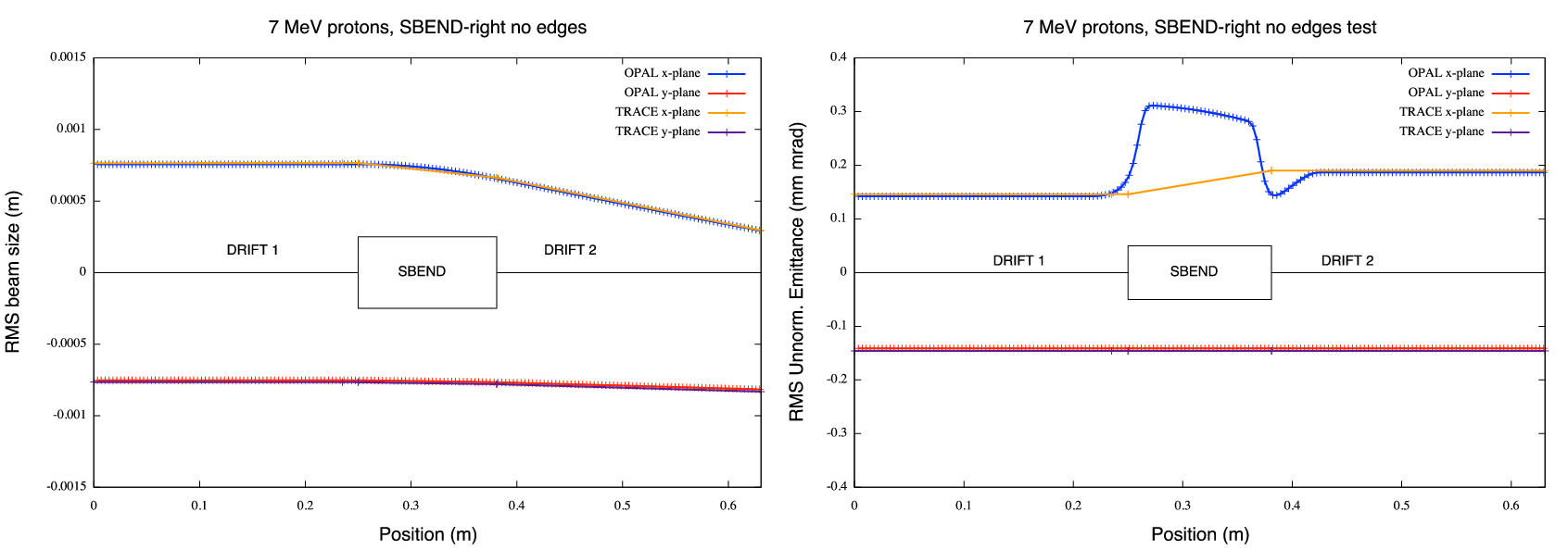 Figure 57. TRACE 3D and OPAL comparison: SBEND without edge angles,
A good overall agreement has been found between the two codes in term of beam size and emittance. The different behavior inside the bending magnet for the horizontal emittance is still undergoing study and it’s probably due to a diverse coordinate system in the two codes.
-
SBEND with edge angles:
// Bending magnet configuration:
K1=0.0,
E1=10*Pi/180.0, E2=5* Pi/180.0,
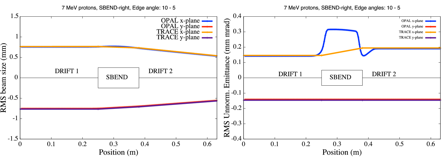 Figure 58. TRACE 3D and OPAL comparison: SBEND with edge angles
Even in this case, a good overall agreement has been found between the two codes in term of beam size and emittance.
-
SBEND with field index:
The field index parameter K1 is defined as:
\[ K1 = \frac{1}{B\rho}\frac{\partial B_y}{\partial x}, \]RBend (OPAL-t). Instead, in TRACE 3D the field index parameter n is:
\[ n = -\frac{\rho}{B_y}\frac{\partial B_y}{\partial x}. \]In order to have a significant focusing effect on both transverse planes, the transport line has been simulated in TRACE 3D using \(n = 1.5\). Since, a different definition exists between OPAL and TRACE 3D on the field index, the n-parameter translation in OPAL language has been done with the following tests:
-
TEST 1: K1 \(=\) n/\(\rho^2\)
-
TEST 2: K1 \(=\) n
-
TEST 3: K1 \(=\) n/\(\rho\)
Only the TEST 2 reports a reasonable behavior on the beam size and emittance, as shown in Figure 59 using:
// Bending magnet configuration:
K1=1.5
E1=0, E2=0,
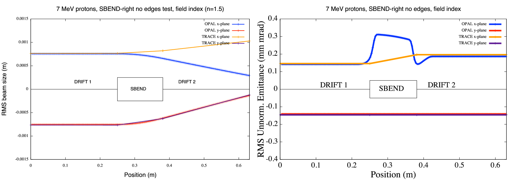 Figure 59. TRACE 3D and OPAL comparison: SBEND with field index and default field map
Concerning the emittances and vertical beam size, a perfect agreement has been found, instead a defocusing effect appears in the horizontal plane. These results have been obtained with the default field map provided by OPAL. However, a better result, only in the beam size as shown in Figure 60, is achieved using a test field map in which the fringe field extension has been changed in the thin lens approximation.
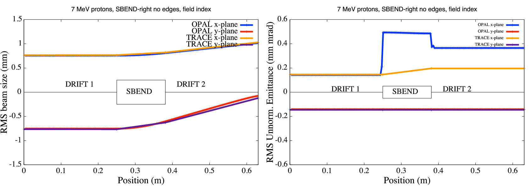 Figure 60. TRACE 3D and OPAL comparison: SBEND with field index and test field map
-
From TRACE 3D to OPAL-t
| Parameter | Trace 3D | OPAL-t |
|---|---|---|
Bend card |
8 |
|
Angle |
Input parameter [deg] |
Input/Calc. parameter [rad] |
Magn. field |
Calculated. [T] |
Input/Calc parameter [T] |
Radius of curv. |
Input parameter [mm] |
Output information [m] |
Field-index |
Input parameter |
Input parameter |
Length |
Calculated [mm] |
Input/Calc parameter [m] |
Length type |
Effective |
Straight |
Edge card |
9 |
|
Edge angle |
Input parameter [deg] |
Input parameter [rad] |
Vertical gap |
9 |
|
Gap |
Total [mm] |
Total [m] |
Fringe field card |
9 |
FIELD MAP |
\(K_1\) |
Default: 0.45 |
- |
\(K_2\) |
Default: 2.8 |
- |
Bend direction |
Bend angle sign |
Coord. rotation |
Horiz. right |
Angle \(>\) 0 |
Angle \(>\) 0 |
Horiz. left |
Angle \(<\) 0 |
Angle \(<\) 0 |
Vertical bend |
Card 8, vf \(>\) 0 |
Coord. rotation |
E.1.12. Conclusion
-
TRACE 3D and TRANSPORT:
-
a perfect agreement has been found between these two codes in transversal envelope and emittance;
-
changing the TRANSPORT units, the input beam parameters, in terms of sigma-matrix coefficients, can directly be imported from TRACE 3D file.
-
-
TRACE 3D and OPAL-t:
-
a good agreement has been found between these two codes in case of sector bending magnet with and without edge angles;
-
the default magnetic field map seems not working properly if the field index is not zero
-
an improvement of the test map used is needed in order to match the TRACE 3D emittance see Figure 60.
-
E.2. Hard Edge Dipole Comparison with ELEGANT
E.2.1. OPAL Dipole
When defining a dipole (SBEND or RBEND) in OPAL, a fringe field
map which defines the range of the field and the Enge coefficients is
required. If no map is provided, the code uses a default map. Here is a
dipole definition using the default map:
      bend1: SBEND, ANGLE = bend_angle,
      E1 = 0, E2 = 0,
      FMAPFN = "1DPROFILE1-DEFAULT",
      ELEMEDGE = drift_before_bend,
      DESIGNENERGY = bend_energy,
      L = bend_length,
      WAKEF = FS_CSR_WAKE;
Please refer to 1DProfile1 for the definition of the field map
and the default map 1DPROFILE1-DEFAULT. It defines a fringe field that
extends to 10 cm away from a dipole edge in both directions and it has
both \(B_y\) and \(B_z\) components. This makes the
comparison between OPAL and other codes which uses a hard edge dipole
by default,cumbersome because one needs to carefully integrate thought
the fringe field region in OPAL in order to come up with the
integrated fringe field value (FINT in ELEGANT) that usually used by
these codes, e.g. the ELEGANT and the TRACE3D. So we need to find a
default map for the hard edge dipole in OPAL.
E.2.2. Map for Hard Edge Dipole
The proposed default map for a hard edge dipole can be:
1DProfile1  0  0  2
-0.00000001 0.0 0.00000001 3
-0.00000001 0.0 0.00000001 3
-99.9
-99.9
On the first line, the two zeros following 1DProfile1 are the orders
of the Enge coefficient for the entrance and exit edge of the dipole.
\(2 cm\) is the default dipole gap width. The second line
defines the fringe field region of the entrance edge of the dipole which
extends from \(-0.00000001 cm\) to
\(0.00000001 cm\). The third line defines the same fringe
field region for the exit edge of the dipole. The \(3\)s on
both line don’t mean anything, they are just placeholders. On the fourth
and fifth line, the zeroth order Enge coefficients for both edges are
given. Since they are large negative numbers, the field in the fringe
field region has no \(B_z\) component and its
\(B_y\) component is just like the field in the middle of the
dipole.
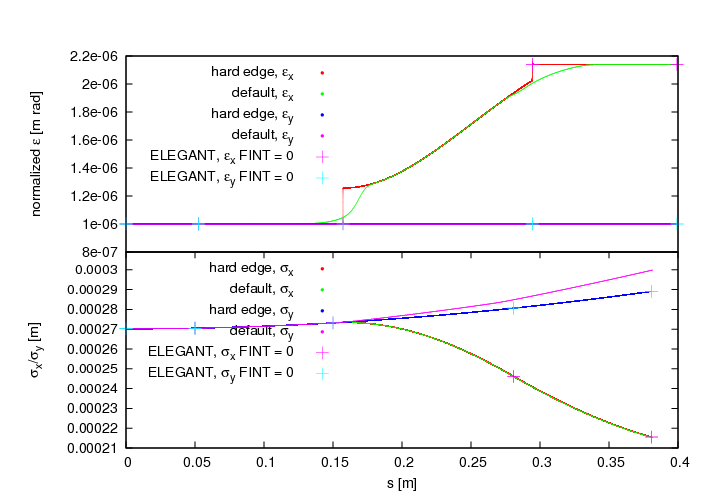
Figure 61 compares the emittances and beam sizes obtained by using the hard edge map, the default map and the ELEGANT. One can see that the results produced by the hard edge map match the ELEGANT results when FINT is set to zero.
E.2.3. Integration Time Step
When the hard edge map is used for a dipole, finer integration time step is needed to ensure the accurate of the calculation. Figure 62 compares the normalized emittances generated using the hard edge map in OPAL with varying time steps to those from the ELEGANT. 0.01ps seems to be a optimal time step for the fringe field region. To speed up the simulations, one can use larger time steps outside the fringe field regions. In Figure 62, one can observe a discontinuity in the horizontal emittance when the hard edge map is used in the calculation. This discontinuity comes from the fact that OPAL emittance is calculated at an instant time. Once the beam or part of the beam gets into the dipole, its \(P_x\) gets a kick which will result in a sudden emittance change.
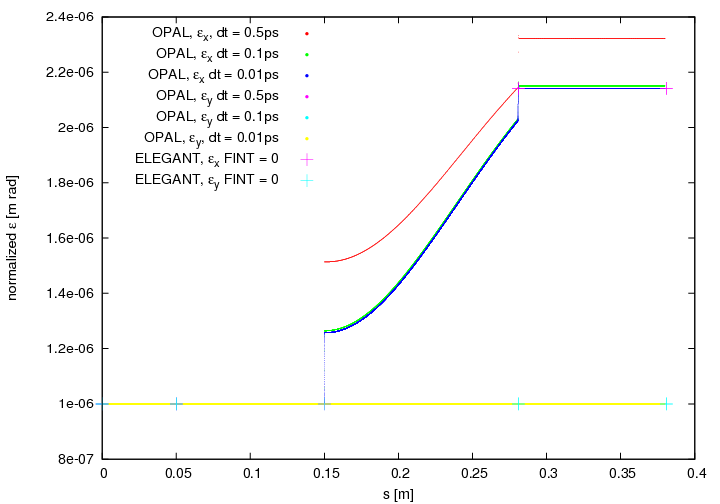
Figure 63 and Figure 64 examine the effects of the fringe field range and the integration time step on the simulation accuracy. Figure 64 is a zoom-in plot of Figure 63. We can conclude that the size of the integration time step has more influence on the accuracy of the simulation.
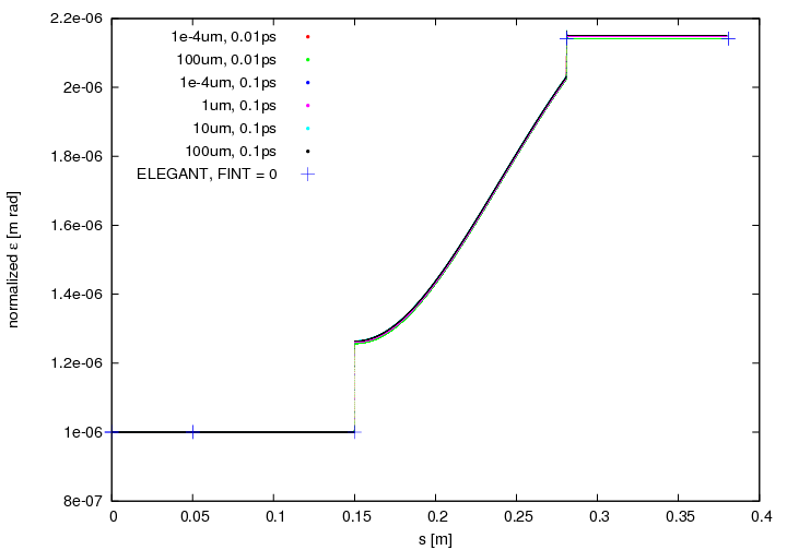
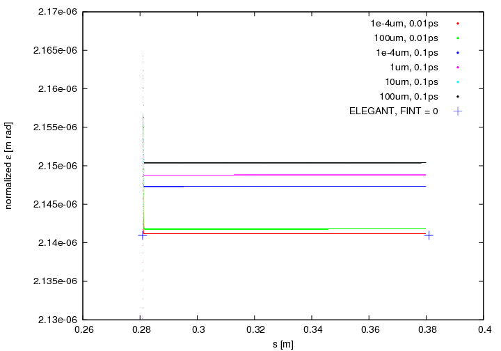
E.3. 1D CSR comparison with ELEGANT
1D-CSR wake function can now be used for the drift element by defining
its attribute WAKEF = FS_CSR_WAKE. In order to calculate the CSR
effect correctly, the drift has to follow a bending magnet whose CSR
calculation is also turned on.
      bend1: SBEND, ANGLE = bend_angle,
      E1 = 0, E2 = 0,
      FMAPFN = "1DPROFILE1-DEFAULT",
      ELEMEDGE = drift_before_bend,
      DESIGNENERGY = bend_energy,
      L = bend_length,
      WAKEF = FS_CSR_WAKE;
       drift1: DRIFT, L=0.4, ELEMEDGE = drift_before_bend +
       bend_length, WAKEF = FS_CSR_WAKE;
E.3.1. Benchmark
The OPAL dipoles all have fringe fields. When comparisons are done between OPAL and ELEGANT [72] for example, one needs to appropriately set the FINT attribute of the bending magnet in ELEGANT in order to represent the field correctly. Although ELEGANT tracks in the (\(x, x', y, y', s, \delta\)) phase space, where \(\delta = \frac{\Delta p}{p_0}\) and \(p_0\) is the momentum of the reference particle, the watch point output beam distributions from the ELEGANT are list in (\(x, x', y, y', t, \beta\gamma\)). If one wants to compare ELEGANT watch point output distribution to OPAL, unit conversion needs to be performed, i.e.
To benchmark the CSR effect, we set up a simple beamline with 0.1 m drift, 30 degree sbend and a 0.4 m drift. When the CSR effect is turn off, Figure 65 shows that the normalized emittances calculated using both OPAL and ELEGANT agree. The emittance values from OPAL are obtained from the .stat file, while for ELEGANT, the transverse emittances are obtained from the sigma output file (enx, and eny), the longitudinal emittance is calculated using the watch point beam distribution output.
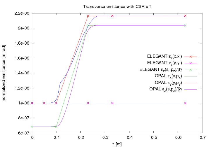
When CSR calculations are enabled for both the bending magnet and the following drift, Figure 66 shows the average \(\delta\) or \(\frac{\Delta p}{p}\) change along the beam line, and Figure 67 compares the normalized transverse and longitudinal emittances obtained by these two codes. The average \(\frac{\Delta p}{p}\) can be found in the centroid output file (Cdelta) from ELEGANT, while in OPAL, one can calculate it using \(\frac{\Delta p}{p} = \frac{1}{\beta^2}\frac{\Delta \overline{E}}{\overline{E}+mc^2}\), where \(\Delta \overline{E}\) is the average kinetic energy from the .stat output file.
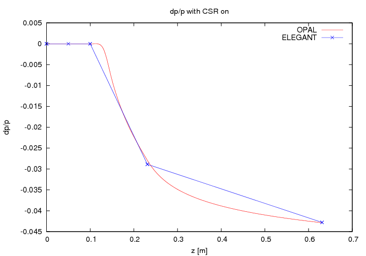
In the drift space following the bending magnet, the CSR effects are calculated using Stupakov’s algorithm with the same setting in both codes. The average fractional momentum change \(\frac{\Delta p}{p}\) and the longitudinal emittance show good agreements between these codes. However, they produce different horizontal emittances as indicated in Figure 67.
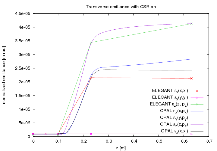
One important effect to notice is that in the drift space following the bending magnet, the normalized emittance \(\epsilon_x(x, P_x)\) output by OPAL keeps increasing while the trace-like emittance \(\epsilon_x(x, x')\) calculated by ELEGANT does not. This can be explained by the fact that with a relatively large energy spread (about \(3\%\) at the end of the dipole due to CSR), a correlation between transverse position and energy can build up in a drift thereby induce emittance growth. However, this effect can only be observed in the normalized emittance calculated with \(\epsilon_x(x, P_x) = \sqrt{\langle x^2 \rangle \langle P_x^2\rangle - \langle xP_x \rangle^2}\) where \(P_x = \beta\gamma x'\), not the trace-like emittance which is calculated as \(\epsilon_x (x, x') = \beta \gamma \sqrt{\langle x^2 \rangle \langle x' {}^{2} \rangle - \langle xx' \rangle^2}\) [prstab2003]. In Figure 67, a trace-like horizontal emittance is also calcualted for the OPAL output beam distributions. Like the ELEGANT result, this trace-like emittance doesn’t grow in the drift. However, their differences come from the ELEGANT’s lack of CSR effect in the fringe field region.
E.4. OPAL & Impact-t
This benchmark compares rms quantities such as beam size and emittance
of OPAL and Impact-t [qiang2005, qiang2006-1, qiang2006-2]. A cold
10mA H+ bunch is expanding in a 1m drift space. A Gaussian distribution,
with a cut at 4 \(\sigma\) is used. The charge is computed by
assuming a 1MHz structure i.e.
\(Q_{\text{tot}}=\frac{I}{\nu_{\text{rf}}}\). For the
simulation we use a grid with \(16^{3}\) grid point and open
boundary condition. The number of macro particles is
\(N_{\text{p}} = 10^{5}\).
E.4.1. OPAL Input
OPTION, ECHO = FALSE, PSDUMPFREQ = 10,
STATDUMPFREQ = 10, REPARTFREQ = 1000,
PSDUMPFRAME = GLOBAL, VERSION=10600;

TITLE, string="Gaussian bunch drift test";

REAL Edes    = 0.001;        // GeV
REAL CURRENT = 0.01;  // A

REAL gamma=(Edes+PMASS)/PMASS;
REAL beta=sqrt(1-(1/gamma^2));
REAL gambet=gamma*beta;
REAL P0 = gamma*beta*PMASS;

D1: DRIFT, ELEMEDGE = 0.0, L = 1.0;

L1: LINE = (D1);

Fs1: FIELDSOLVER, FSTYPE = FFT, MX = 16, MY = 16, MT = 16, BBOXINCR=0.1;

Dist1: DISTRIBUTION, TYPE = GAUSS,
       OFFSETX = 0.0, OFFSETY = 0.0, OFFSETZ = 15.0e-3,
       SIGMAX = 5.0e-3, SIGMAY = 5.0e-3, SIGMAZ = 5.0e-3,
       OFFSETPX = 0.0, OFFSETPY = 0.0, OFFSETPZ = 0.0,
       SIGMAPX = 0.0 , SIGMAPY = 0.0 , SIGMAPZ = 0.0 ,
       CORRX = 0.0, CORRY = 0.0, CORRZ = 0.0,
       CUTOFFX = 4.0, CUTOFFY = 4.0, CUTOFFLONG = 4.0;

Beam1: BEAM, PARTICLE = PROTON, CHARGE = 1.0, BFREQ = 1.0, PC = P0,
               NPART = 1E5, BCURRENT = CURRENT, FIELDSOLVER = Fs1;

SELECT, LINE = L1;

TRACK, LINE = L1, BEAM = Beam1, MAXSTEPS = 1000, ZSTOP = 1.0, DT = 1.0e-10;
 RUN, METHOD = "PARALLEL-T", BEAM = Beam1, FIELDSOLVER = Fs1, DISTRIBUTION = Dist1;
ENDTRACK;
STOP;
E.4.2. Impact-t Input
!Welcome to Impact-t input file.
!All comment lines start with "!" as the first character of the line.
! col row
1 1
!
! information needed by the integrator:
! step-size, number of steps, and number of bunches/bins (??)
!
!   dt    Ntstep  Nbunch
1.0e-10   700     1
!
! phase-space dimension, number of particles, a series of flags
! that set the type of integrator, error study, diagnostics, and
! image charge, and the cutoff distance for the image charge
!
! PSdim  Nptcl   integF  errF  diagF  imchgF  imgCutOff (m)
6 100000  1 0 1 0 0.016
!
! information about mesh: number of points in x, y, and z, type
! of boundary conditions, transverse aperture size (m),
! and longitudinal domain size (m)
!
!  Nx  Ny  Nz  bcF   Rx    Ry    Lz
16 16 16 1 0.15 0.15 1.0e5
!
!
! distribution type number (2 == Gauss), restart flag, space-charge substep
! flag, number of emission steps, and max emission time
!
! distType  restartF  substepF  Nemission  Temission
2           0         0         -1          0.0
!
!  sig*   sigp*  mu*p*  *scale  p*scale  xmu*      xmu*
!
0.005 0.0 0.0  1. 1. 0.0 0.0
0.005 0.0 0.0  1. 1. 0.0 0.0
0.005 0.0 0.0  1. 1. 0.0 0.0462
!
! information about the beam: current, kinetic energy, particle
! rest energy, particle charge, scale frequency, and initial cavity phase
!
! I/A   Ek/eV     Mc2/eV          Q/e  freq/Hz  phs/rad
0.010   1.0e6     938.271998e+06  1.0  1.0e6      0.0
!
!
! ======= machine description starts here =======
! the following lines, which must each be terminated with a '/',
! describe one beam-line element per line; the basic structure is
! element length, ???, ???, element type, and then a sequence of
! at most 24 numbers describing the element properties
!   0  drift tube    2      zedge radius
!   1  quadrupole    9      zedge, quad grad, fileID,
!                             radius, alignment error x, y
!                             rotation error x, y, z
! L/m  N/A N/A  type  location of starting edge  v1  <B0><B0><B0>  v23 /
1.0    0   0    0    0.0                           0.5            /
E.4.3. Results
A good agreement is shown in the
Figure 68 and Figure 69. This proves to some extend
the compatibility of the space charge solvers of OPAL and Impact-t.
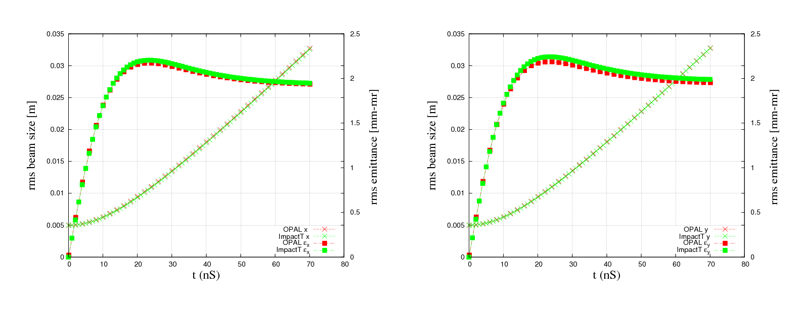
Impact-t and OPAL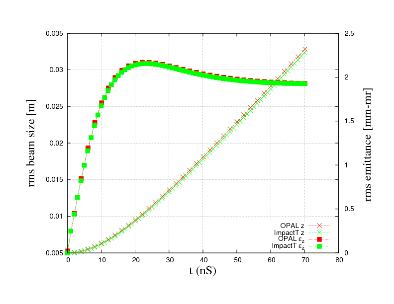
Impact-t and OPALE.5. References
[68] K. Crandall and D. Rusthoi, Documentation for TRACE: An Interactive Beam-Transport Code, Tech. Rep. LA—10235-MS, Los Alamos National Laboratory (1985).
[69] K. L. Brown et al., TRANSPORT - A Computer Program for Designing Charged Particle Beam Transport Systems, Tech. Rep. CERN 80-4, European Organization for Nuclear Research (1980).
[70] U. Rohrer, PSI graphic transport framework based on a CERN-SLAC-FERMILAB version by K.L. Brown et al.
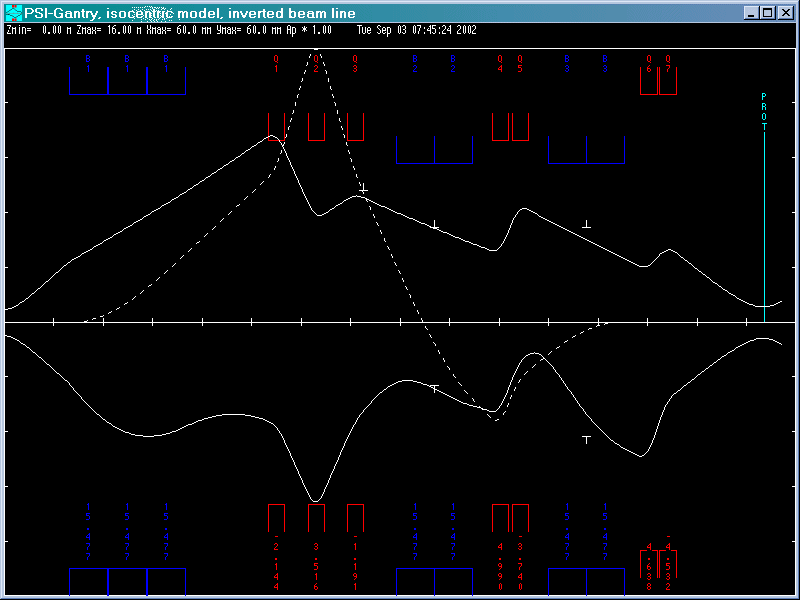
[72] M. Borland, elegant: a flexible SDDS-compliant code for accelerator simulation, Tech. Rep. LS-287, Advanced Photon Source (2000).